library(fpp3);
library(patchwork);
library(ggfortify);11 Introduction to Time Series Regressions
Time series data are observations of variables made repeatedly over time, often at regular intervals (annually, quarterly, monthly, daily,…). The main issue with regressions with time series data is that the observations generally cannot be thought of as independent draws from a population. As you will see as this chapter progresses, the presence of intertemporal correlations, trends and other features can lead to a wide range of problems in regression analysis, if not properly addressed.
We use the following packages in this chapter, plus a few others.
There are a number of time-series object types in R. We will primarily use the tsibble object type provided by the fpp3 package. The fpp3 package includes a number of the packages we have been using, plus a few additional ones which help in the analysis of time series. See Hyndman and Athanasopoulos (2021), Hyndman and Athanasopoulos (2023). The tsibble is a time-series version of the tibble object type. We will occasionally use the ts object type provided in base R. The following example creates a vector of random numbers and converts it into a ts object, then converts it into a tsibble object.
set.seed(13)
x <- rnorm(12,0,1)
x.ts <- ts(x, start=c(1990,1),freq=4) #Define as Quarterly data starting at 1990Q1
x.ts
Qtr1 Qtr2 Qtr3 Qtr4
1990 0.5543269 -0.2802719 1.7751634 0.1873201
1991 1.1425261 0.4155261 1.2295066 0.2366797
1992 -0.3653828 1.1051443 -1.0935940 0.4618709x.tsbl <- as_tsibble(x.ts)
x.tsbl# A tsibble: 12 x 2 [1Q]
index value
<qtr> <dbl>
1 1990 Q1 0.554
2 1990 Q2 -0.280
3 1990 Q3 1.78
4 1990 Q4 0.187
5 1991 Q1 1.14
6 1991 Q2 0.416
7 1991 Q3 1.23
8 1991 Q4 0.237
9 1992 Q1 -0.365
10 1992 Q2 1.11
11 1992 Q3 -1.09
12 1992 Q4 0.462Data frames can be converted directly to tsibbles. We do this in the upcoming example, where the Period column in the data frame is first converted to a yearmonth object, and set as the index of the tsibble.
11.1 Overview
Many economic time series display cyclical behavior, such as in panel (a) of Fig. 11.1, which shows the time series plot of the quarterly series \(Y\) from the dataset ts_02.xlsx. Cyclical behavior implies “serial correlation” (a.k.a. “autocorrelation”) meaning that \(\mathrm{cov}[Y_{t},Y_{t-k}] \neq 0\) for some \(k \neq 0\). The scatterplot in panel (b) of \(Y_{t}\) against \(Y_{t-1}\) shows that consecutive observations are very highly correlated. By definition, i.i.d. observations cannot display serial correlation.
ts02 <- readxl::read_excel("data\\ts_02.xlsx") %>%
        mutate(Period=yearquarter(Period), Y_1=lag(Y,1)) %>%
        as_tsibble(index=Period)
p1 <- ts02 %>% autoplot(Y) + theme_minimal() + xlab("")
p2 <- ts02 %>% ggplot(aes(x=Y_1, y=Y), size=0.5) + geom_point() + theme_minimal() +
               ylab("Y(t)") + xlab("Y(t-1)")
(p1 | p2) + plot_layout(widths=c(1.5,1)) + plot_annotation(tag_levels="a")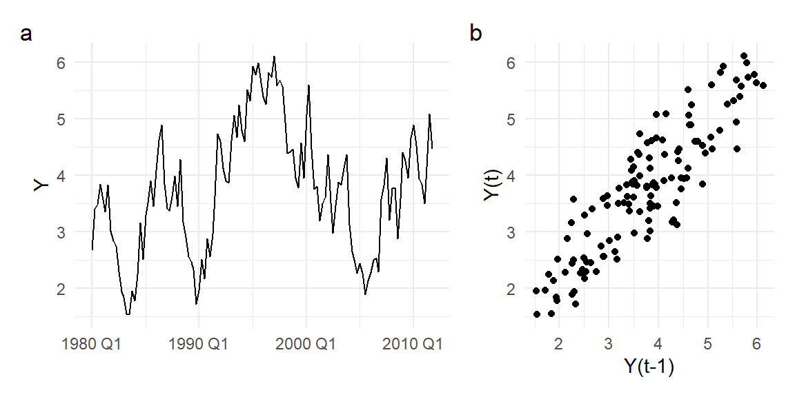
Economic time series often also display features such as trends and seasonality. Panel (a) of Fig. 11.2 shows a plot of Singapore’s monthly Industrial Production Index from 1983M1 to 2017M12, data in ts_01.xlsx. The upward trend seems the most dominant feature, though cyclical deviations from trend are also obvious. The size of the fluctuations are also increasing over time, which is not unusual in upward trending economic time series. Seasonality – repetitive patterns that occur with regular periods – is also present. We zoom in on the sub-period 1990M1 to 1995M12 in Fig 2(b) where there seasonality is easier to see. There appears to be an annual pattern, with a sharp drop near the start of the year (usually in February) followed by a sharp positive response in the following month.
ts01 <- readxl::read_excel("data\\ts_01.xlsx") %>%
        select(DATE, IP_SG) %>%
        mutate(DATE=yearmonth(DATE)) %>%
        as_tsibble(index=DATE)
p1 <- ts01 %>%
      autoplot(IP_SG) + theme_minimal() + xlab("")
p2 <- ts01 %>%
      filter(DATE>=yearmonth("1990M1") & DATE<=yearmonth("1995M12")) %>%
      autoplot(IP_SG) + theme_minimal() + xlab("")
(p1 | p2) + plot_annotation(tag_levels="a")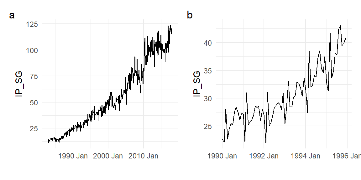
11.2 Some Simple Time Series Models
We first discuss some basic tools for time series analysis, and a few simple time series models for cycles, trends and seasonality, so that we have a vocabulary for discussing such features and their consequences.
11.2.1 Transformations
We often apply some sort of transformation to a time series prior to analysis. For instances, we might work with the log of the time series rather than the series itself. Since the log function is strictly increasing, this does not affect the sign of the period-to-period changes in the time series. But as the log function is strictly-concave, applying a log-transformation attenuates fluctuations in the series, with larger fluctuations receiving greater attenuation. Log transformations therefore help to control the tendency of fluctuations in trending time series to increase over time. Log transformations also linearize exponential trends, which is common in economic time series. Fig. 11.3 shows the log transformed IP_SG.
p3 <- ts01 %>% autoplot(log(IP_SG)) + theme_minimal() + xlab("")
p3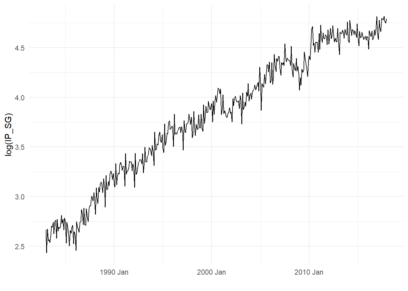
Yet another advantage of the log transformation is that period-to-period percentage changes can be approximated by the first difference of log-transformed data (the “log-difference”): \[ \frac{Y_{t} - Y_{t-1}}{Y_{t-1}} \approx \ln Y_{t} - \ln Y_{t-1}\,. \] This arises from the first-order linear approximation of the log function around \(Y_{t-1}\). Alternatively, the log-difference can be interpreted as a continuous growth rate.
11.2.2 Sample Autocorrelation Function
We can summarize the serial correlation (or autocorrelation) in a time series by calculating its sample autocorrelation function. Given a time series \(Y_{t}\), \(t=1,2,...,T\), define the sample autocovariance function to be \[ \hat{\gamma}_{k} = \frac{1}{T}\sum_{t=k+1}^{T} (Y_{t}-\overline{Y})(Y_{t-k}-\overline{Y}) \,,\, k=0,1,2,... \] where \(\overline{Y}\) is the sample mean defined in the usual way. This is, of course, just the usual sample covariance formula, except that here we measure a variable’s covariance with itself at some lag. Note that the summation index starts at \(t=k+1\) instead of \(t=1\), because we need to take \(k\) lags of the variable. Despite only adding up \(T-k\) terms, we divide by \(T\) instead of \(T-k\) (we won’t get into the reasons why here). This is called a sample autocovariance function because we are computing the sample autocovariances at \(k=0,1,2,...\), (i.e., we have a function of \(k\)). The sample autocovariance of \(Y_{t}\) at lag \(0\) is just the sample variance of \(Y_t\). Finally, the sample autocorrelation function is defined as \[ \hat{\rho}_{k} = \frac{\hat{\gamma}_{k}}{\hat{\gamma}_{0}}. \] Fig. 11.4 shows the sample acf for the \(Y_{t}\) series shown in Fig. 11.1. The dotted bands are the \(\pm 1.96\) standard errors of the sample acf, which helps us to determine significance of the autocorrelations. We see that the autocorrelations of this series decline as we consider observations further apart.
p1 <- ts02 %>% ACF(Y) %>% autoplot() + ylim(c(-1,1)) + theme_minimal()
p1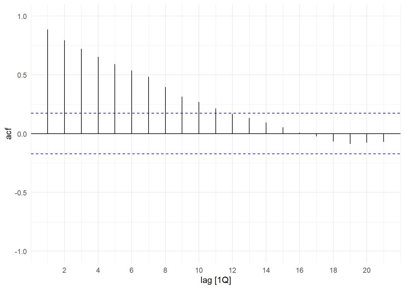
11.2.3 Trend
There are a number of ways to model trend. We can model a trending series as a “deterministic trend” process such as \[ Y_{t} = \beta_0 + \beta_1 t + \epsilon_{t}\,,t=1,2,...,T \,, \tag{11.1}\] where for the moment we take \(\epsilon_{t}\) to be some zero-mean i.i.d. noise term. Here we indicate dates as an integer series, although this might represent some regular period like months or quarters. We can use any deterministic function of \(t\) for the trend. For example we can have a quadratic deterministic trend \[ Y_{t} = \beta_0 + \beta_1 t + \beta_2 t^2 + \epsilon_{t}\,,t=1,2,...,T\,. \tag{11.2}\] We fit using OLS the quadratic deterministic trend model to the log(IP_SG) series. The fitted line and the residuals are shown in Fig. 11.5.
ts01 <- ts01 %>% mutate(t=1:length(ts01$IP_SG), tsq = t^2)
mdl_dqt <- lm(log(IP_SG) ~ t + tsq, data=ts01)
mdl_dqt %>% summary() %>% coef()
df_plot <- ts01 %>% mutate("Fitted"=fitted(mdl_dqt), "Residuals"=residuals(mdl_dqt))
p1 <- autoplot(df_plot, log(IP_SG), size=0.5) +
      autolayer(df_plot, Fitted) + theme_minimal() + xlab("")
p2 <- autoplot(df_plot, Residuals) + theme_minimal() + xlab("")
(p1 | p2) + plot_annotation(tag_levels = 'a')
Estimate Std. Error t value Pr(>|t|)
(Intercept) 2.519434e+00 1.529628e-02 164.70896 0.000000e+00
t 7.774090e-03 1.677910e-04 46.33197 1.517867e-166
tsq -5.833467e-06 3.859553e-07 -15.11436 1.812010e-41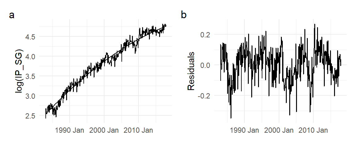
Of course, no series is likely to be a pure deterministic trend plus iid noise. In Fig. 11.5(b), the residuals display cycles and seasonality, and can be thought of as a de-trended version of the Industrial Production series. Sometimes the purpose of estimating a trend is precisely to obtain a de-trended series, so we can focus on the remaining components.
Instead of specifying a particular functional form for the trend, a more flexible way would be to use non-parametric methods. See Appendix A for a description of one such method.
Another way to model trend in a series is to say that on average the series changes every period by some value \(\alpha\), i.e., \[ Y_{t} - Y_{t-1} = \alpha + \epsilon_{t}\,, \] where again for the moment we assume \(\epsilon_{t}\) to be some iid zero-mean noise term. We often denote the first difference \(Y_{t} - Y_{t-1}\) by \(\Delta Y_{t}\). The model above is often written as \[ Y_{t} = \alpha + Y_{t-1} + \epsilon_{t}. \tag{11.3}\] If \(\alpha>0\), then \(Y_{t}\) increases by an average of \(\alpha\) every period, and therefore trends upwards. The process (11.3) is called a random walk with drift if \(\alpha \neq 0\), or a random walk without drift (or simply a “random walk”) if \(\alpha=0\).
There is an essential difference between the random walk approach (11.3) and deterministic trend approaches such as in (11.1) or (11.2). We can better understand (11.3) better by following the process starting from some fixed \(Y_0\). Suppose that the variance of \(\epsilon_{t}\) is \(\sigma^2\). We have \[ \begin{aligned} Y_{1} &= \alpha + Y_{0} + \epsilon_{1} &\mathrm{var}[Y_{1}|Y_{0}] &= \sigma^2\\ Y_{2} &= \alpha + Y_{1} + \epsilon_{2} = Y_{0} + 2\alpha + \epsilon_{1} + \epsilon_{2} &\mathrm{var}[Y_{2}|Y_{0}] &= 2\sigma^2 \\ Y_{3} &= \alpha + Y_{2} + \epsilon_{3} = Y_{0} + 3\alpha + \epsilon_{1} + \epsilon_{2} + \epsilon_{3} &\mathrm{var}[Y_{3}|Y_{0}] &= 3\sigma^2 \\ &\vdots & \vdots &\\ Y_{t} &= \alpha + Y_{t-1} + \epsilon_{t} = Y_{0} + \alpha t + \epsilon_{1} + \epsilon_{2} + \epsilon_{3} + \dots + \epsilon_{t} &\mathrm{var}[Y_{t}|Y_{0}] &= t\sigma^2 \end{aligned} \] We see that if \(Y_{t}\) follows (11.3), then it contains a linear deterministic trend (if \(\alpha \neq 0\)), but unlike the linear deterministic trend process (11.1) there is also an accumulation of noise terms, resulting in a variance that increases steadily over time.
We simulate and plot in Fig. 11.6 one hundred series each of the “pure” linear deterministic trend process (11.1) with \(\beta_0=100\) and \(\beta_1=0.3\) (panel (a)), the random walk with drift (11.3) with \(\alpha=0.3\) (panel (b)), and the “pure” random walk (11.3) with \(\alpha=0\) (panel (c)). In the latter two cases, we start the process off at \(Y_0 = 100\). For all three cases, we set the variance of the noise term at 1, and simulate series of 200 observations.
set.seed(20);
R <- 100; bigT <- 200; b0 <- 100; b1 <- 0.3; a0 <- 0.3; sigma <- 1; Y0 <- 100
dttrnd <-  matrix(rep(0,R*bigT),ncol=R)
rwwd <- rwwod <- dttrnd
timeidx <- 1:bigT
for (r in 1:R){
  epsln <- rnorm(bigT,0,1)
  epscum <- cumsum(epsln)
  dttrnd[,r] <- b0 + b1*timeidx + epsln
  rwwd[,r] <- 100 + a0*timeidx + epscum
  rwwod[,r] <- 100 + epscum
}
theme1 <- theme_minimal() + theme(legend.position = "none")
p1 <- dttrnd %>% as.ts() %>% autoplot(facets=F, size=0.5) +
      ggtitle("Det. Trend") + ylim(c(50,200)) + theme1
p2 <- rwwd %>% as.ts() %>% autoplot(facets=F, size=0.5) +
      ggtitle("RW with drift") + ylim(c(50,200)) + theme1
p3 <- rwwod %>% as.ts() %>% autoplot(facets=F, size=0.5) +
      ggtitle("RW without drift") + ylim(c(50,200)) + theme1
(p1 | p2 | p3) + plot_annotation(tag_levels = 'a')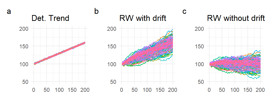
Because the ‘pure’ deterministic trend process is simply a deterministic function of \(t\) plus a non-accumulating noise term, such a process is very predictable. The random walk with drift, while trending upwards, is much less predictable because of the increasing variance. The random walk without drift has no tendency to trend upwards, but also shows increasing variance.
Despite not containing a deterministic trend, the increasing variance in the random walk without drift means that in any finite sample one can observe a wide range of behaviors, including outcomes that appear to trend upwards or downwards, despite the fact that the average period-to-period growth rate is zero. Fig. 11.7 shows a few series drawn from the 200 simulations in panel (c) of Fig. 11.6. We refer to this behavior, which comes about because of the increasing variance, as the “stochastic trend”.
rwwod[,c(15, 20, 40, 65, 70, 95)] %>% as.ts() %>% autoplot(facet=F) + theme1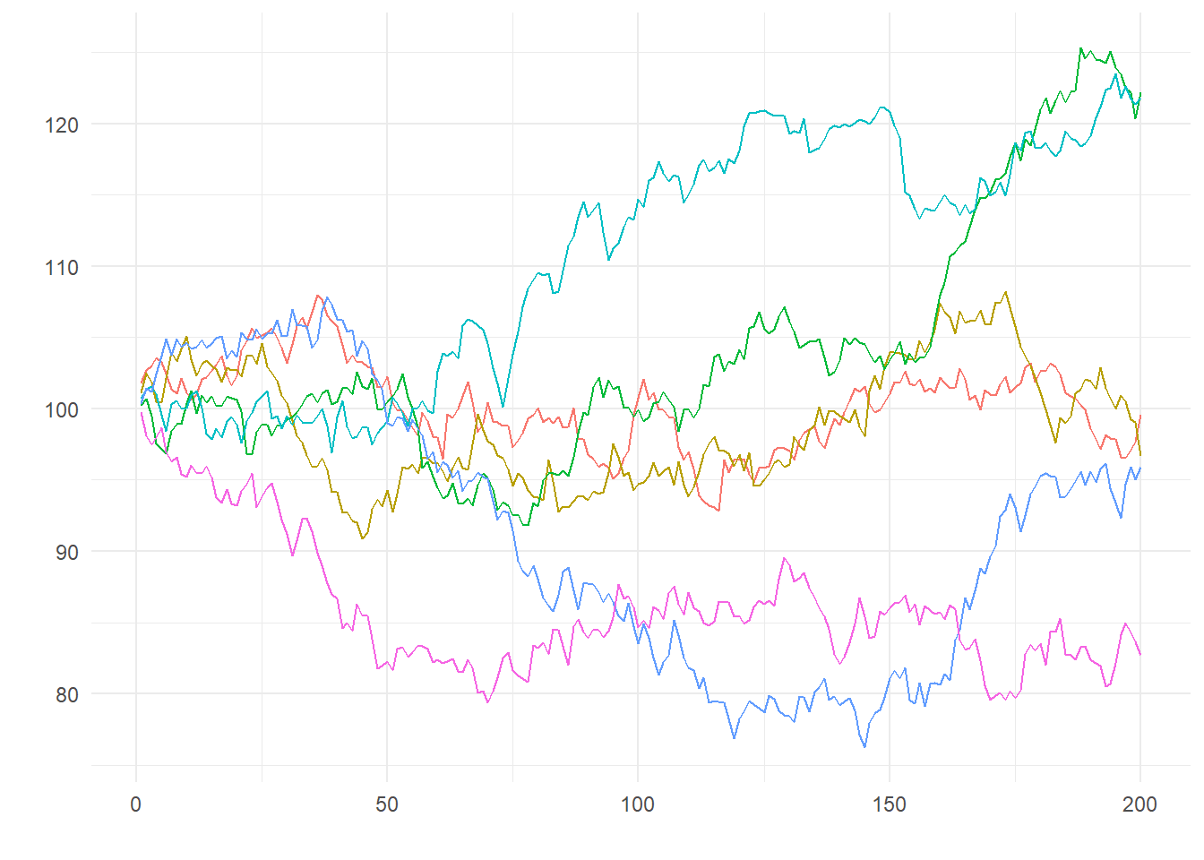
In the random walk with drift, we have both the linear deterministic trend (due to the non-zero \(\alpha\)) and the accumulating errors that lead to increasing variances. We refer to the linear deterministic trend part as the “drift” (hence the name “random walk with drift”), and the “increasing variance” part as the “stochastic trend”. The parameter \(\alpha\) is called the drift parameter.
Deterministic Trend: \(\quad Y_{t} = f(t) + \epsilon_{t}\).
Random Walk: \[ Y_{t} = \alpha + Y_{t-1} + \epsilon_{t} = \underbrace{\quad Y_{0} + \alpha t\quad}_{\text{linear det. trend}} + \underbrace{\;\sum_{t=1}^{T} \epsilon_{t}\;}_{\text{stoc. trend}} \,, \] “with drift” if \(\alpha \neq 0\), “without drift” otherwise.
We can estimate \(\alpha\) in the random walk with drift simply as the sample mean of \(\Delta Y_{t}\). We estimate this for the log(IP_SG) model below.
a0 <- mean(diff(log(ts01$IP_SG)))
df_plot2 <- ts01 %>% mutate(Fitted=lag(log(IP_SG))+a0, Residuals=log(IP_SG)-Fitted)
p1 <- autoplot(df_plot2, log(IP_SG), size=0.5) +
      autolayer(df_plot2, Fitted) + theme_minimal() + xlab("")
p2 <- autoplot(df_plot2, Residuals) + theme_minimal() + xlab("")
(p1 | p2) + plot_annotation(tag_levels = 'a')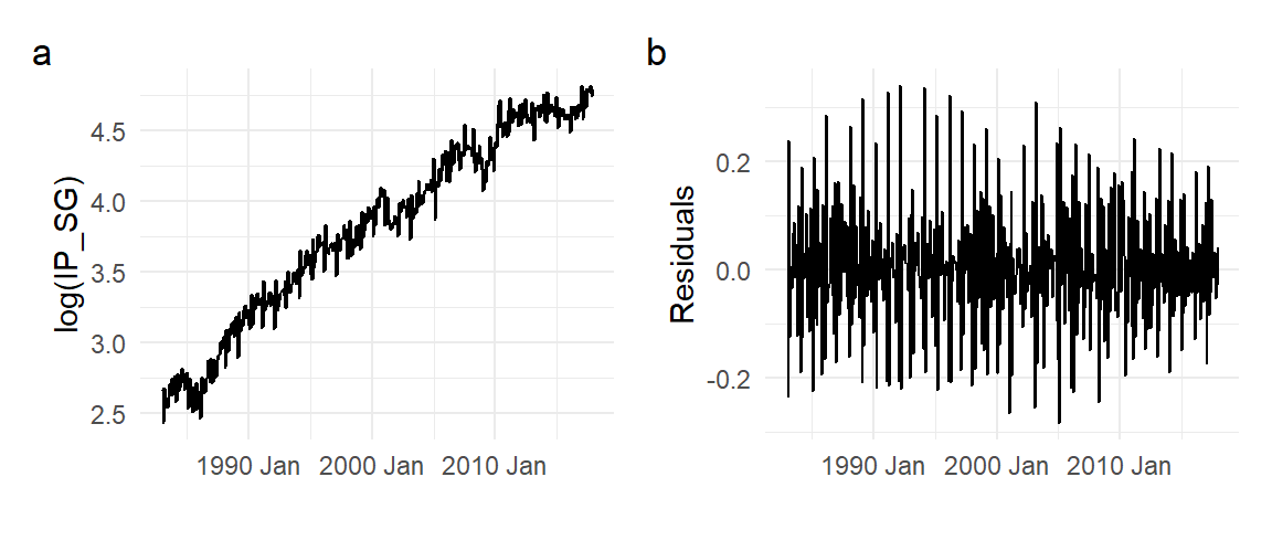
It is hard to make out the actual log(IP_SG) and the fitted values in Fig. 11.8. We zoom in on a subsample in Fig. 11.9. The fitted values appear to be simply the lagged actual values. By construction, the fitted values are the lagged values plus the estimated growth rate \(\hat{\alpha}\).
df_plot2sub <- df_plot2 %>%
  filter(DATE>=yearmonth("1990M1") & DATE<=yearmonth("1995M12"))
autoplot(df_plot2sub,log(IP_SG)) + autolayer(df_plot2sub, Fitted, size=1) +
  theme_minimal() + xlab("")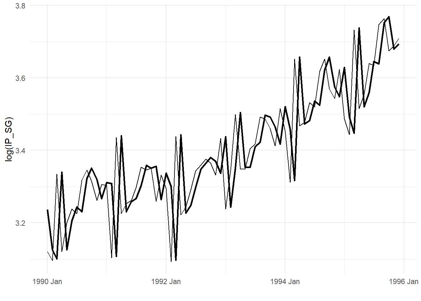
To remove the stochastic trend and drift from a random walk process, simply take the first difference \(\Delta Y_{t} = Y_{t} - Y_{t-1}\), or take the residuals from the fitted random walk model as in Fig. 11.8. In the latter the estimated growth rate is also removed.
While we have taken \(\epsilon_{t}\) to be i.i.d., for the moment, this will not be the case in most applications. We see in the residuals in Fig. 11.8 that there is seasonality, and less prominently, some cyclical patterns in the monthly growth rates.
Incidentally, trends show up in the sample acf as highly persistent autocorrelation. The following is the sample acf of the log(IP_SG) series.
ts01 %>% ACF(log(IP_SG)) %>% autoplot() + ylim(c(-1,1)) + theme_minimal()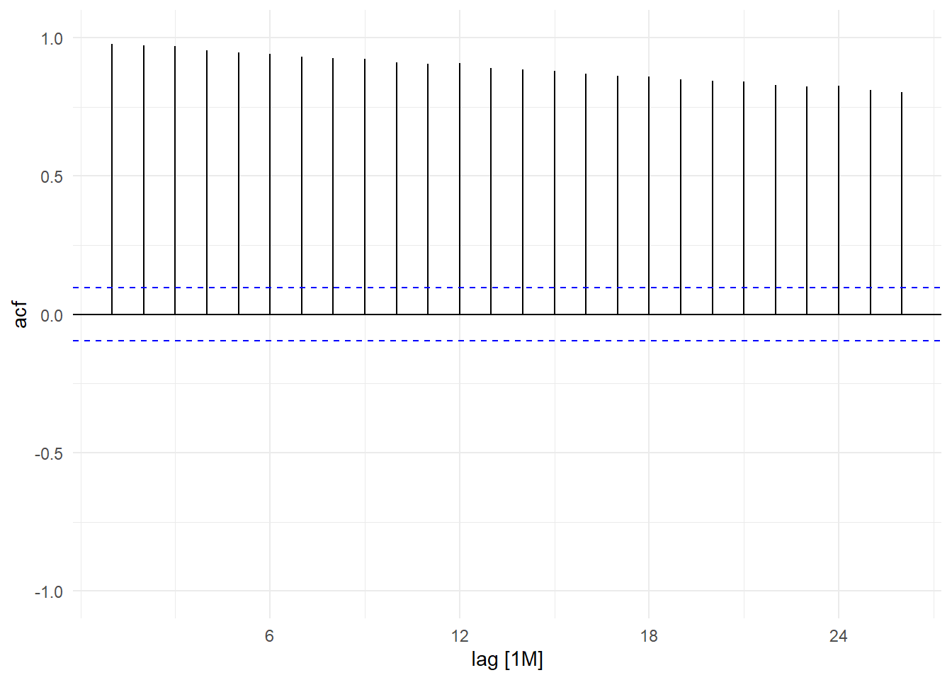
Stochastic trends, even without drift, are also highly persistent processes. The following is the sample acf of one of the simulated random walks without drift that was shown in Fig. 11.6(c).
rwwod[,20] %>% as.ts() %>% as_tsibble() %>% ACF(value) %>%
  autoplot() + ylim(c(-1,1)) + theme_minimal() + xlab("lags")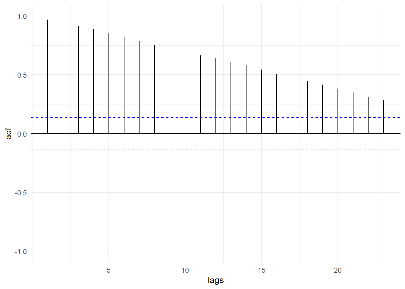
We set aside for a later chapter the question of how to detect the presence of stochastic trend in a data series.
11.2.4 Seasonality
Seasonals are patterns that occur with regular periods, often for ‘mechanical’ reasons, such as housing starts always being higher in the summer than in the winter, or tourist arrivals systematically peaking in the summer and at the end of the year.
Fig. 11.12 shows the “seasonal plot” for the IP_SG growth rate, as measured by the first difference of the log-transformed IP_SG series. We see that there is a very regular annual down-up-down pattern in industrial production growth over the Feb-Apr period, arising from the fewer number of calendar days in February, together with the Chinese New Year holidays which usually happen in February.
ts01 %>% gg_season(difference(log(IP_SG)), labels = "both") + theme_minimal()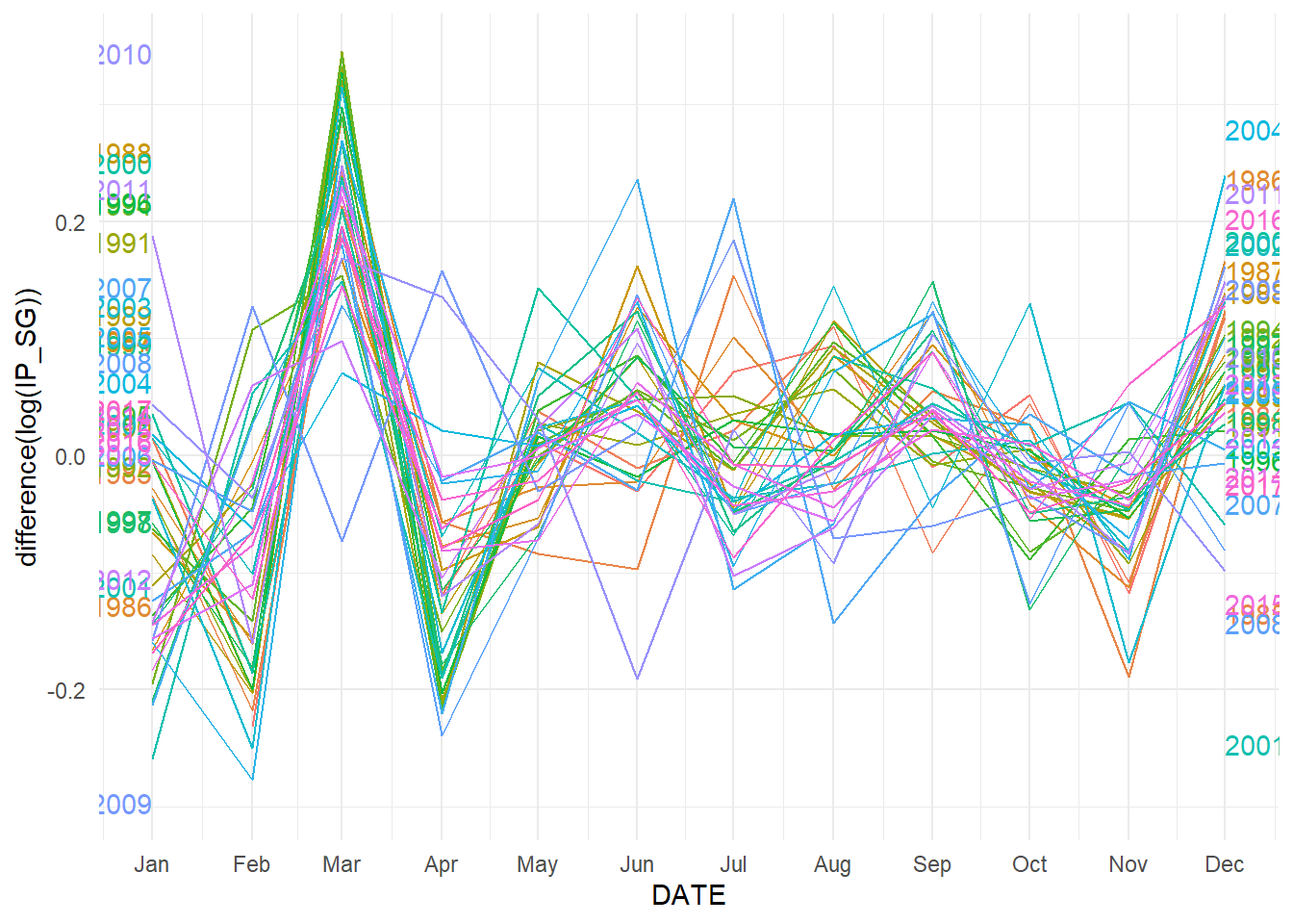
Seasonality can also show up in the sample acf of a series. Fig. 11.13 shows the sample acf of the IP_SG growth rate series.
ts01 %>% ACF(difference(log(IP_SG)), lag_max=48) %>% autoplot() +
      ylim(c(-1,1)) + theme_minimal()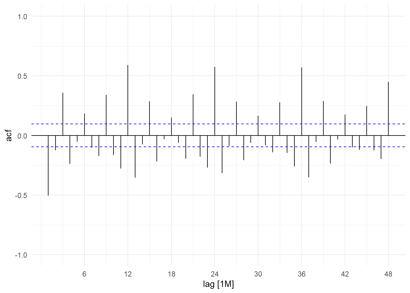
Seasonality shows up as significant autocorrelations at multiples of the “seasonal lag”, which for monthly data is 12. These ‘seasonal spikes’ did not show up in the sample acf of trending log(IP_SG) series in Fig. 11.10 because the seasonality (and all other features of the series) was overwhelmed by the trend, which is the dominant feature.
One way of modelling seasonal data is by using seasonal indicator variables (a.k.a. “seasonal dummy variables” or “seasonal dummies”). For monthly data, these are binary variables marking the month of the observation: the January dummy variable takes ‘1’ for all January observations, ‘0’ for all other observations; the February dummy variable takes ‘1’ for all February observations, ‘0’ for all others, and so on. The following 12 columns show the first 18 observations for each of the twelve monthly seasonal dummies for the IP_SG data series.
ts01 <- ts01 %>%
  mutate(d01=ifelse(month(DATE)==1,1,0),
         d02=ifelse(month(DATE)==2,1,0),
         d03=ifelse(month(DATE)==3,1,0),
         d04=ifelse(month(DATE)==4,1,0),
         d05=ifelse(month(DATE)==5,1,0),
         d06=ifelse(month(DATE)==6,1,0),
         d07=ifelse(month(DATE)==7,1,0),
         d08=ifelse(month(DATE)==8,1,0),
         d09=ifelse(month(DATE)==9,1,0),
         d10=ifelse(month(DATE)==10,1,0),
         d11=ifelse(month(DATE)==11,1,0),
         d12=ifelse(month(DATE)==12,1,0))
ts01 %>% select(d01,d02,d03,d04,d05,d06,d07,d08,d09,d10,d11,d12) %>%
  filter(DATE>=yearmonth("1985M1") & DATE<=yearmonth("1986M6")) %>%
knitr::kable()| d01 | d02 | d03 | d04 | d05 | d06 | d07 | d08 | d09 | d10 | d11 | d12 | DATE |
|---|---|---|---|---|---|---|---|---|---|---|---|---|
| 1 | 0 | 0 | 0 | 0 | 0 | 0 | 0 | 0 | 0 | 0 | 0 | 1985 Jan |
| 0 | 1 | 0 | 0 | 0 | 0 | 0 | 0 | 0 | 0 | 0 | 0 | 1985 Feb |
| 0 | 0 | 1 | 0 | 0 | 0 | 0 | 0 | 0 | 0 | 0 | 0 | 1985 Mar |
| 0 | 0 | 0 | 1 | 0 | 0 | 0 | 0 | 0 | 0 | 0 | 0 | 1985 Apr |
| 0 | 0 | 0 | 0 | 1 | 0 | 0 | 0 | 0 | 0 | 0 | 0 | 1985 May |
| 0 | 0 | 0 | 0 | 0 | 1 | 0 | 0 | 0 | 0 | 0 | 0 | 1985 Jun |
| 0 | 0 | 0 | 0 | 0 | 0 | 1 | 0 | 0 | 0 | 0 | 0 | 1985 Jul |
| 0 | 0 | 0 | 0 | 0 | 0 | 0 | 1 | 0 | 0 | 0 | 0 | 1985 Aug |
| 0 | 0 | 0 | 0 | 0 | 0 | 0 | 0 | 1 | 0 | 0 | 0 | 1985 Sep |
| 0 | 0 | 0 | 0 | 0 | 0 | 0 | 0 | 0 | 1 | 0 | 0 | 1985 Oct |
| 0 | 0 | 0 | 0 | 0 | 0 | 0 | 0 | 0 | 0 | 1 | 0 | 1985 Nov |
| 0 | 0 | 0 | 0 | 0 | 0 | 0 | 0 | 0 | 0 | 0 | 1 | 1985 Dec |
| 1 | 0 | 0 | 0 | 0 | 0 | 0 | 0 | 0 | 0 | 0 | 0 | 1986 Jan |
| 0 | 1 | 0 | 0 | 0 | 0 | 0 | 0 | 0 | 0 | 0 | 0 | 1986 Feb |
| 0 | 0 | 1 | 0 | 0 | 0 | 0 | 0 | 0 | 0 | 0 | 0 | 1986 Mar |
| 0 | 0 | 0 | 1 | 0 | 0 | 0 | 0 | 0 | 0 | 0 | 0 | 1986 Apr |
| 0 | 0 | 0 | 0 | 1 | 0 | 0 | 0 | 0 | 0 | 0 | 0 | 1986 May |
| 0 | 0 | 0 | 0 | 0 | 1 | 0 | 0 | 0 | 0 | 0 | 0 | 1986 Jun |
We can model seasonality with seasonal dummies using the specification \[ Y_{t} = \beta_{1} d_{1,t} + \beta_{2} d_{2,t} + \dots + \beta_{12} d_{12,t} + \epsilon_{t} \tag{11.4}\] where \(d_{1,t}\) is the January dummy, \(d_{2,t}\) is the February dummy, and so on, and where we again (for the moment) take \(\epsilon_{t}\) to be a zero-mean iid noise term. This specification allows the mean of \(Y_{t}\) to depend on the ‘season’ (in this case, the month). For January observations, only \(d_{1,t}=1\), the other dummies are zero, therefore \(\mathrm{E}[Y_{t}] = \beta_{1}\) for January observations. For February observations, only \(d_{2,t}=1\), the other dummies are zero, therefore \(\mathrm{E}[Y_{t}] = \beta_{2}\) for February observations, and so on.
Notice there is no intercept term in (11.4). This is because all of the dummies add up to a vector of ones. Including a constant will result in perfect collinearity (this is known as the dummy variable trap). If we wish to include the intercept, we will have to drop one of the dummy variables, as in (11.5) below, where we drop the January dummy. \[ Y_{t} = \alpha_{0} + \alpha_{2} d_{2,t} + \dots + \alpha_{12} d_{12,t} + \epsilon_{t} \tag{11.5}\] This changes the interpretation of the coefficients slightly. The parameter \(\alpha_0\) is now the January mean of \(Y_{t}\) and serves as the reference month. The February mean of \(Y_{t}\) is now \(\alpha_0 + \alpha_2\), so \(\alpha_2\) is the difference between the February mean and the January mean. The other coefficients are interpreted similarly. We explore yet another equivalent specification in the exercises.
The seasonal dummies can be used in conjunction with other models we have discussed so far. For instance, we can have a quadratic deterministic trend model with seasonal dummies: \[ Y_{t} = \alpha_{0} + \alpha_{2} d_{2,t} + \dots + \alpha_{12} d_{12,t} + \beta_{1}t + \beta_{2}t^2 + \epsilon_{t} \tag{11.6}\] We fit (11.6) to the log(IP_SG) model using OLS; the fitted values and residuals are shown in Fig. 11.14.
## recall we have previously added t and the seasonal dummies to ts01
mdl_dqt <- lm(log(IP_SG)~t+tsq+d02+d03+d04+d05+d06+d07+d08+d09+d10+d11+d12, data=ts01)
mdl_dqt %>% summary() %>% coef()
df_plot1 <- ts01 %>% mutate("Fitted"=fitted(mdl_dqt), "Residuals"=residuals(mdl_dqt))
p1 <- autoplot(df_plot1, log(IP_SG), size=0.5) +
      autolayer(df_plot1, Fitted) + theme_minimal() + xlab("")
p2 <- autoplot(df_plot1, Residuals) + theme_minimal() + xlab("")
(p1 | p2) +   plot_annotation(tag_levels = 'a')
Estimate Std. Error t value Pr(>|t|)
(Intercept) 2.490454e+00 1.965402e-02 126.71473330 0.000000e+00
t 7.768060e-03 1.455858e-04 53.35728414 1.456574e-185
tsq -5.832981e-06 3.348699e-07 -17.41864454 3.794588e-51
d02 -1.013478e-01 2.156942e-02 -4.69868204 3.590501e-06
d03 1.131723e-01 2.156951e-02 5.24686286 2.497552e-07
d04 -6.292830e-04 2.156967e-02 -0.02917445 9.767398e-01
d05 -2.884859e-03 2.156988e-02 -0.13374479 8.936707e-01
d06 4.298396e-02 2.157016e-02 1.99275152 4.695768e-02
d07 3.467546e-02 2.157049e-02 1.60754144 1.087130e-01
d08 4.523024e-02 2.157089e-02 2.09681856 3.662779e-02
d09 8.296558e-02 2.157135e-02 3.84610093 1.393025e-04
d10 5.959898e-02 2.157187e-02 2.76281065 5.991151e-03
d11 6.966586e-03 2.157245e-02 0.32293906 7.469076e-01
d12 8.191373e-02 2.157309e-02 3.79703297 1.687982e-04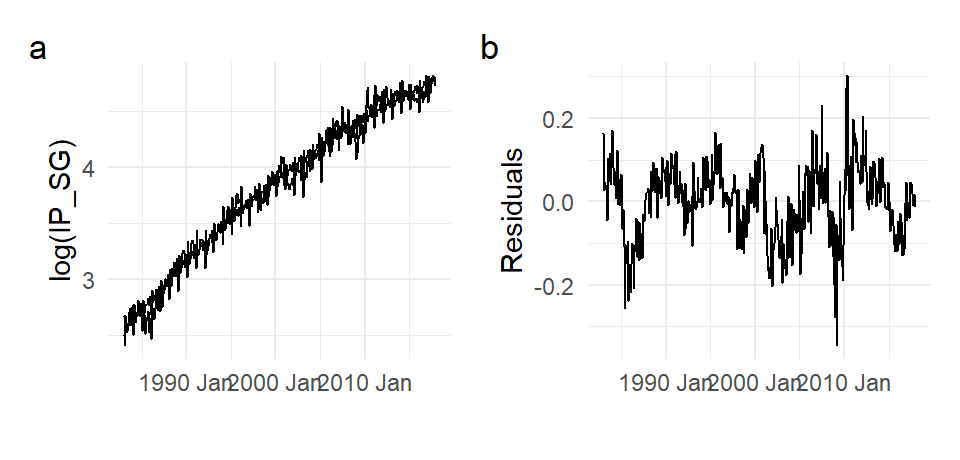
Fig. 11.15 zooms in on a subsample of the fit. The residuals in Fig. 11.14 can be thought of as de-trended “seasonally-adjusted” log(IP_SG).
df_plot1sub <- df_plot1 %>%
  filter(DATE>=yearmonth("1990M1") & DATE<=yearmonth("2000M12"))
autoplot(df_plot1sub,log(IP_SG)) + autolayer(df_plot1sub, Fitted, size=1) +
  theme_minimal() + xlab("")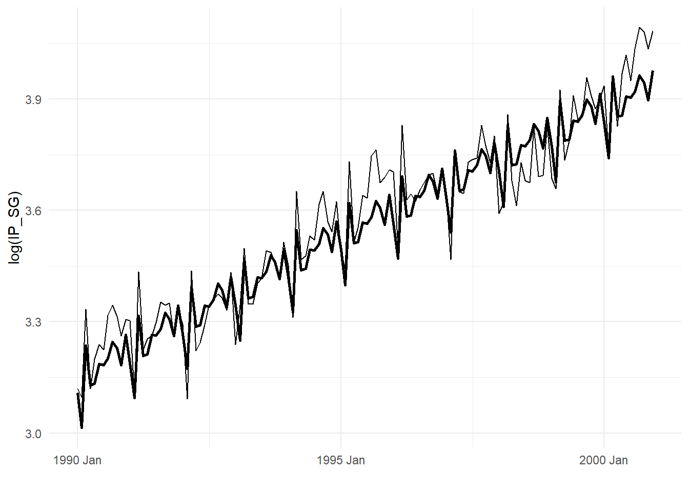
We can also fit a random walk with seasonal dummies by fitting the seasonal dummy model to the first differences: \[ Y_{t} - Y_{t-1} = \alpha_0 + \alpha_{2} d_{2,t} + \dots + \alpha_{12} d_{12,t} + \epsilon_{t}\,. \tag{11.7}\] The fitted values can be obtained as \[ \hat{Y}_{t} = Y_{t-1} + \hat{\alpha}_0 + \hat{\alpha}_{2} d_{2,t} + \dots + \hat{\alpha}_{12} d_{12,t}\;,\; t=2,3,...,T\,. \] We fit this model to the log(IP_SG series), output shown below; fitted values and residuals are shown in Fig. 11.16. Fig. 11.17 zooms in on a smaller subsample. Presumably after removing trend and seasonality, only cyclical behavior remains. Notice that what we get after detrending and seasonal adjustment can look very different, depending on what we assume about the trend and how we de-seasonalize. Compare Fig. 11.14(b) and Fig. 11.16(b).
ts01a <- ts01 %>% mutate(lIP_SG=lag(IP_SG),
                         dlIP_SG=log(IP_SG)-log(lIP_SG)) %>% filter(DATE>=yearmonth("1985M2"))
mdl_rwseas <- lm(dlIP_SG~d02+d03+d04+d05+d06+d07+d09+d10+d11+d12, data=ts01a)
df_plot2 <- ts01a %>% mutate(Fitted=log(lIP_SG)+fitted(mdl_rwseas),
                             Residuals=log(IP_SG)-Fitted)
p1 <- autoplot(df_plot2, log(IP_SG), size=0.5) +
      autolayer(df_plot2, Fitted) + theme_minimal() + xlab("")
p2 <- autoplot(df_plot2, Residuals) + theme_minimal() + xlab("")
(p1 | p2)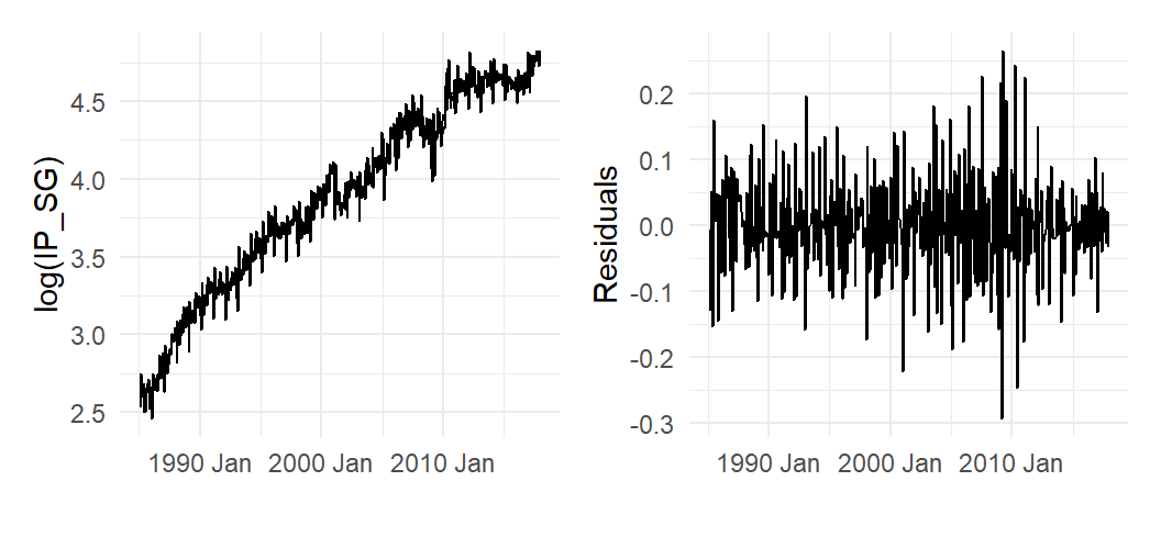
df_plot2sub <- df_plot2 %>%
  filter(DATE>=yearmonth("1990M1") & DATE<=yearmonth("1995M12"))
autoplot(df_plot2sub,log(IP_SG)) + autolayer(df_plot2sub, Fitted, size=1) +
  theme_minimal() + xlab("") +
  plot_annotation(subtitle="Fig 17. log(IP_SG) Actual and Fitted (bold), subsample")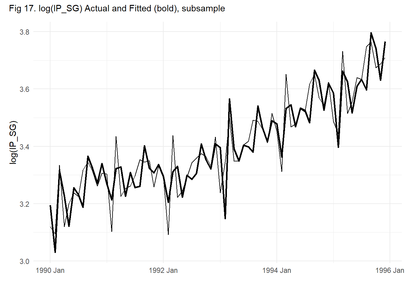
There are other ways to model seasonality. For instance, we can consider a “seasonal random walk”, which for monthly data would be \[ Y_{t} = Y_{t-12} + \epsilon_{t}. \] This sort of seasonality can be dealt with by taking ‘seasonal differences’, i.e., \(\Delta_{12}Y_{t} = Y_{t} - Y_{t-12}\). This is in fact a fairly common approach when dealing with seasonal data.
Seasonally-adjusted (s.a.) versions of time series are often provided by official statistics agencies, sometimes together with the Non-Seasonally Adjusted (n.s.a.) versions, sometimes in place of it. Seasonal adjustment is often done by first estimating a “trend-cycle” (using sophisticated versions of the moving average method described in Appendix A), then estimating the seasonal component from the series with trend-cycle removed. This results in a decomposition of the original series into a trend-cycle component, a seasonal component, and an ‘irregular’ component. The seasonally-adjusted version of the data is obtained by removing the seasonal component from the original.
We apply one such method (called “X-11”) to log(IP_SG), with default settings. Fig. 11.18 shows the decomposition of log(IP_SG) into its various components, and Fig. 11.19 shows the original and seasonally adjusted series.1 Panel (b) zooms in on a sub-sample to better illustrate the seasonally adjusted series. It also highlights that care is needed when using default settings. The early year seasonal pattern in IP_SG is driven by the Chinese New Year holidays, which typically occurs in February. Occasionally it falls in January, as it did in 1993. This might lead to what appears to be big ‘shocks’ where there were only moderate ones.
ipsg_dcmp <- ts01 %>% model(x11=X_13ARIMA_SEATS(log(IP_SG) ~ x11())) %>% components()
autoplot(ipsg_dcmp) + theme_minimal()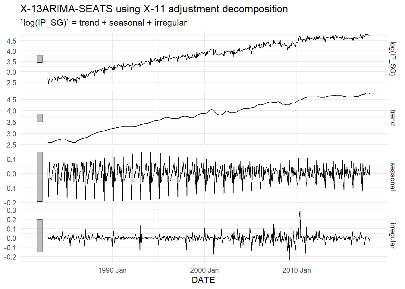
p2 <- ipsg_dcmp %>%
  ggplot(aes(x = DATE)) +
  geom_line(aes(y = `log(IP_SG)`), size=0.5) +
  geom_line(aes(y = season_adjust), size=1) + theme_minimal()
p3 <- ipsg_dcmp %>%
  filter(DATE>=yearmonth("1990M1") & DATE<=yearmonth("1995M12")) %>%
  ggplot(aes(x = DATE)) +
  geom_line(aes(y = `log(IP_SG)`), size=0.5) +
  geom_line(aes(y = season_adjust), size=1) + theme_minimal()
(p2 | p3) + plot_annotation(tag_levels = "a")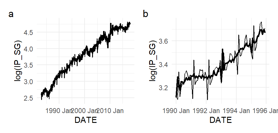
11.2.5 Cycles
Cycles are somewhat harder to define, and we will not attempt a definition here. Instead we will focus on serial correlation or autocorrelation, which as we pointed out earlier, can manifest as cyclical behavior in a time series. Returning to the series that was displayed in Fig. 11.1, the scatterplot in Fig. 11.1(b) suggested that perhaps a model such as \[ Y_{t} = \beta_{0} + \beta_{1} Y_{t-1} + \epsilon_{t} \tag{11.8}\] may describe the behavior of the series well. Such a process is called an Autoregression of Order 1, or AR(1). In fact, the series in Fig. 11.1 was simulated from such a model, with \(\epsilon_{t}\) as some i.i.d. noise term.
One will recognize the Random Walk as an example of such an AR(1), with \(\beta_1=1\), and we saw that such a process will have a stochastic trend, and also a drift if \(\beta_{0} \neq 0\). However, if \(-1 < \beta_1 < 1\), then the AR(1) in (11.8) behaves quite differently. The following is another simulation of such a series, with \(\beta_{1} = 0.7\). This time we simulate a lengthy series, to illustrate a point about such series.
simAR <- function(a0, a1, bigT){
  burn = 100
  Z <- rep(0,bigT+burn)
  u <- rnorm(bigT+burn,0,1)
  for (t in 2:(bigT+burn)){
    Z[t] <- a0 + a1*Z[t-1] + u[t]
  }
  return(Z[(burn+1):(burn+bigT)])
}
set.seed(13)
bigT=1000; a0 = 1; a1 = 0.8
X <- simAR(a0,a1,bigT)
dfplot <- data.frame(t=(1:bigT),X=X)
dfplot %>% ggplot() + geom_line(aes(x=t,y=X)) + theme_minimal()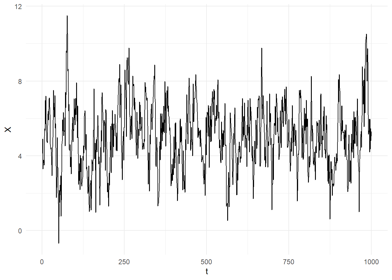
There are cycles in this series of the boom-bust form (because we set \(\beta_{1}\) between zero and one), though the period and amplitude of each ‘cycle’ is not regular. Notice also that the series fluctuates around some constant value, and the overall size of the fluctuations appear fairly stable. In Fig. 11.21, we plot the sample acf for the full sample, as well as for three subsamples. We notice that the sample autocorrelations die off fairly quickly. Also, we see that the sample acf is very stable over the entire sample. This should be unsurprising, since the time series was simulated from a single model across the 1000 observations.
X <- as_tsibble(as.ts(X, freq=1))
Xearly <- X %>% filter(index>=1 & index<=300)
Xmiddle <- X %>% filter(index>=351 & index<=650)
Xlate <- X %>% filter(index>=700 & index<=1000)
p1 <- ACF(X,value,lag_max=16) %>% autoplot() + ylim(c(-1,1)) + theme_minimal()
p2 <- ACF(Xearly,value,lag_max=16) %>% autoplot() + ylim(c(-1,1)) + theme_minimal()
p3 <- ACF(Xmiddle,value,lag_max=16) %>% autoplot() + ylim(c(-1,1)) + theme_minimal()
p4 <- ACF(Xlate,value,lag_max=16) %>% autoplot() + ylim(c(-1,1)) + theme_minimal()
(p1 | p2) / (p3 | p4)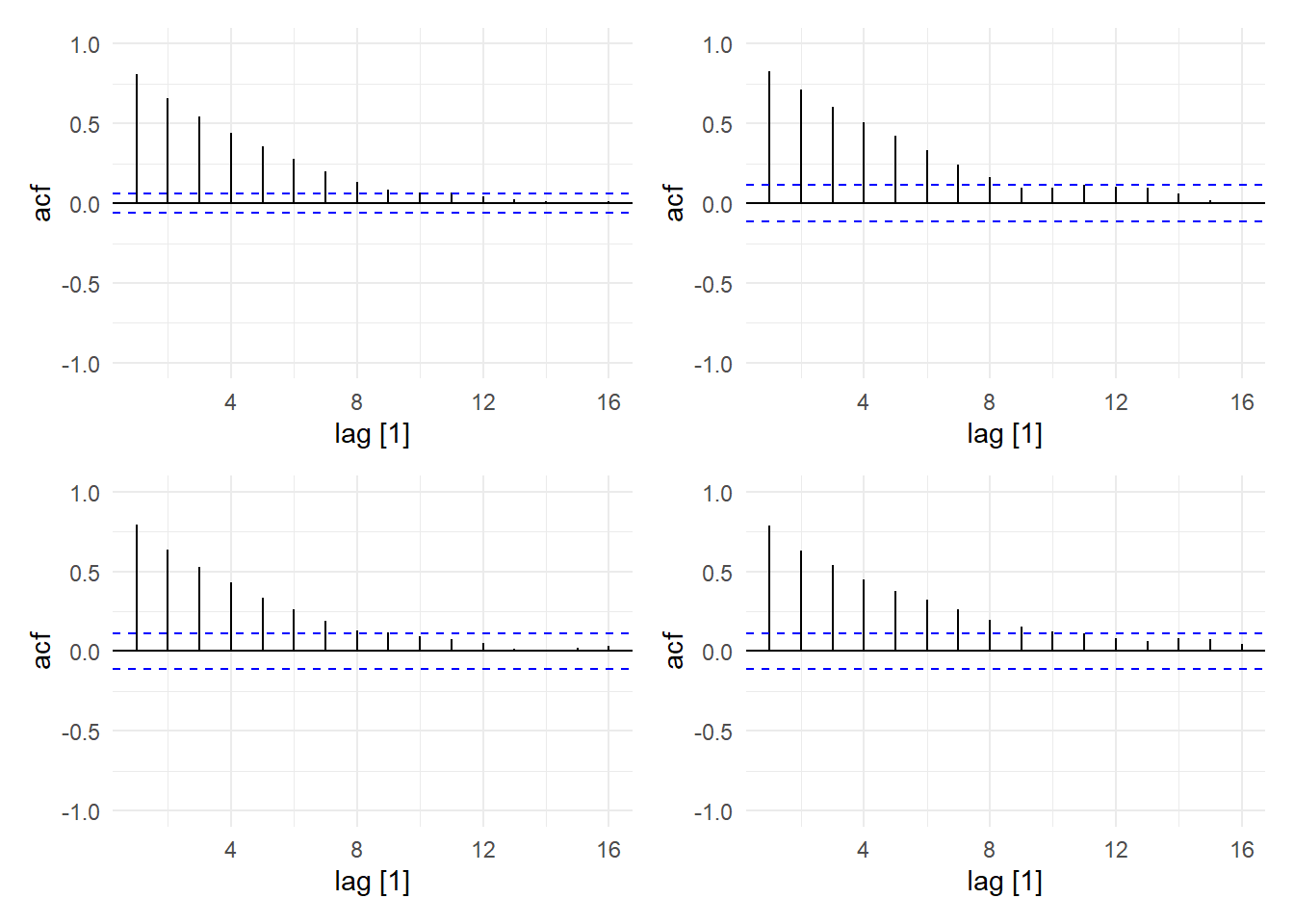
A time series \(Y_{t}\) is said to be covariance-stationary if it has
- a constant and finite mean \(\mathrm{E}[Y_{t}] < \infty\) for all \(t\),
- a constant and finite variance \(\mathrm{var}[Y_{t}] < \infty\) for all \(t\), and
- an autocorrelation function \(\mathrm{cov}[Y_{t},Y_{t-k}]\) that is finite and that may depend on \(k\) but not on \(t\).
Covariance-stationary processes are processes that are “stable” in the sense given in its definition. A process whose autocorrelations dies off reasonably quickly as we consider observations further apart is said to be “weakly dependent”. 2 Processes like the random walk are not weakly dependent, but are “persistent”. Trending processes are not covariance-stationary. Seasonal processes may or may not be stationary, and may or may not be weakly dependent.
11.3 Time Series Regressions
We come now to time series regressions where we have ‘variables’ on the right-hand-side, rather than (only) functions of the time index or dummy variables. For the most part, we will begin by assuming that our variables are covariance-stationary and weakly dependent. If dealing with trending data, we assume that we have made whatever transformations are necessary (e.g., taking first differences, using seasonally-adjusted data) to obtain covariance-stationarity. Later we add deterministic trends and seasonal dummies to the mix.
11.3.1 Dynamic Specifications
We first note that in time series regressions, we have the possibility of including lagged regressors, and also lagged dependent variables into the specification. Of course, we could simply have the “static” specification \[ Y_{t} = \alpha_{0} + \alpha_{1}X_{t} + \epsilon_{t} \;, \] but in general we will want to consider “dynamic” specifications such as the following:
- “Distributed Lag Models”: \[ Y_{t} = \alpha_{0} + \beta_{0} X_{t} + \beta_{1} X_{t-1} + ... \beta_{q} X_{t-q} + \epsilon_{t}\,. \tag{11.9}\] Such models are useful because there is always the possibility that the influence of an explanatory variable may take several periods to fully work out. For instance, the effect of a change in interest rates on inflation may take several quarters to fully take effect. In (11.9), suppose there is a one-period only one-unit shock in \(X_t\). The immediate effect on \(Y_{t}\) is \(\beta_0\), but the affect on \(Y_{t}\) does not end there. Even though this is one-period only impulse in \(X\), there is a lingering effect: the effect on \(Y_{t+1}\) is \(\beta_1\), and that on \(Y_{t+2}\) is \(\beta_2\), and so on. If there is a permanent change in \(X_{t}\) by one unit, then the effect on \(Y_{t}\) is cumulative: the total effect (or “long-run cumulative dynamic multiplier”) is \(\beta_{0} + \beta_{1} + \dots + \beta_{q}\).
It should be noted that even when lags of \(X_t\) are included in the specification, it may well be that the noise term \(\epsilon_{t}\) are still not i.i.d., i.e., there may still be serial correlation in the noise term.
We have already seen the stationary autogressive model of order 1: \[ Y_{t} = \alpha_{0} + \alpha_{1}Y_{t-1} + \epsilon_{t}\,,\,\, |\alpha_1| < 1\,. \] Such models are used primarily to model cyclical dynamics in the data. There may be more than one lag of the dependent variable.
“Autoregressive Distributed Lag (ARDL) models”: \[ Y_{t} = \alpha_{0} + \alpha_{1}Y_{t-1} + \beta_{0} X_{t} + \beta_{1} X_{t-1} + ... + \beta_{q} X_{t-q} + \epsilon_{t}\,. \tag{11.10}\] Such specifications imply an ‘infinite distributed lag structure’ for the effect of \(X_{t}\) or \(Y_{t}\). Since (11.10) is assumed to hold for all \(t\), we have \[ Y_{t-1} = \alpha_{0} + \alpha_{1}Y_{t-2} + \beta_{0} X_{t-1} + \beta_{1} X_{t-2} + ... + \beta_{q} X_{t-q-1} + \epsilon_{t-1}\,. \] Substituting into ( 11.10) gives \[ Y_{t} = \alpha_{0}(1 + \alpha_{1}) + \alpha_{1}^{2}Y_{t-2} + \beta_{0} X_{t} + (\beta_{1} + \alpha_{1} \beta_{0}) X_{t-1} + ... + \alpha_{1}\beta_{q} X_{t-q-1} + \epsilon_{t} + \alpha_{1} \epsilon_{t-1}\,. \] Continuing this process by substituting \(Y_{t-2}\), then \(Y_{t-3}\) and so on, we get the infinite distributed lag structure on \(X_{t}\).
We mentioned for the distributed lag model (11.9) that the noise term may contain cyclical dynamics. There is a close connection between such models and the autoregressive distributed lag specification. Suppose \[ Y_{t} = \alpha_{0} + \beta_{0}X_{t} + \beta_{1} X_{t-1} + u_{t}\,,\, u_{t} = \rho u_{t-1} + \epsilon_{t}\,,\,|\rho| < 1 \tag{11.11}\] where \(\epsilon_{t}\) is iid. This is a model with “covariance-stationary AR(1) errors”. Such models imply an ARDL specification. Since \[ \rho Y_{t-1} = \rho \alpha_{0} + \rho \beta_{0}X_{t-1} + \rho \beta_{1} X_{t-2} + \rho u_{t-1} \,, \tag{11.12}\] subtracting (11.12) from (11.11) gives \[ Y_{t} - \rho Y_{t-1} = \alpha_{0} (1-\rho) + \beta_{0} X_{t} + (\beta_{1} - \rho \beta_{0}) X_{t-1} + \rho \beta_{1}X_{t-2} + u_{t} - \rho u_{t-1} \] i.e., \[ Y_{t} = \alpha_{0} (1-\rho) + \rho Y_{t-1} + \beta_{0} X_{t} + (\beta_{1} - \rho \beta_{0}) X_{t-1} + \rho \beta_{1}X_{t-2} + \epsilon_{t}\,. \] If a dynamic model has i.i.d. errors, we will refer to it as a dynamically correct model. Of course, the dynamic structure in the error term might be much more complicated than a simple AR(1) model, and it may well be that even an ARDL specification might not be sufficient for obtaining a dynamically complete model.
11.3.2 Assumptions
We will write our (potentially dynamic) linear regression as \[ Y_{t} = x_{t}^\mathrm{T}\beta + \epsilon_{t} \] where \(x_{t}\) is a vector of regressors. Although this looks like a static specification, bear in mind that the vector \(x_{t}\) may contain lagged regressors or even lagged dependent variable. E.g., in the ARDL model (11.10), we have \[ x_{t}^{\mathrm{T}} = \begin{bmatrix} 1 & Y_{t-1} & X_{t} & X_{t-1} & \dots & X_{t-q} \end{bmatrix} \] and \[ \beta = \begin{bmatrix} \alpha_{0} & \alpha_{1} & \beta_{0} & \beta_{1} & \dots & \beta_{q} \end{bmatrix}^\mathrm{T}. \]
We will consider the usual OLS assumptions, and how they must be modified for dynamic time series regressions.
First, in cross-sectional regressions we often assume iid draws. As we have already discussed, this is usually an untenable assumption for time series data. We allow for non-iid behavior in our time series, but for the moment, we will assume that the variables in our regression are covariance-stationary and weakly-dependent.
In cross-sectional regressions, we usually assume \(\mathrm{E}[\epsilon_{i} | x_{1}, x_{2}, ..., x_{N}] = 0\). Recall that this is the key assumption for unbiased OLS estimators. For time series regressions this assumption becomes \[ \mathrm{E}[\epsilon_{t} | x_{1}, x_{2}, ..., x_{T}] = 0\,. \tag{11.13}\] We will refer to this assumption as “strong exogeneity”.
It turns out that this assumption is often too strong time series data. For example, take the AR(1) model \[ Y_{t} = \beta_0 + \beta_1 Y_{t-1} +\epsilon_{t}\,,\,t=2,3,...,T \] and suppose \(\epsilon_{t}\) are i.i.d. noise terms. Assumption (Eq. 11.13) then becomes \[ \mathrm{E}[\epsilon_{t} | Y_{1}, Y_{2}, ..., Y_{T-1}] = 0\, \tag{11.14}\] but this is impossible. If \(\epsilon_{t}\) is uncorrelated with \(Y_{t-1}\), then it is definitely correlated with \(Y_t\), whereas (11.14) say that \(\epsilon_{t}\) is uncorrelated with all \(Y_{t}\), \(t=2,...,T\). This argument applies for all specifications with lagged dependent variables. Strong exogeneity cannot hold in any specification that includes a lagged dependent variable as a regressor. Even if you do not have lagged dependent variables, strong exogeneity may still not hold. For instance, you may be forced to omit variables in your equation that can help forecast future outcomes of your regressor. Strong exogeneity will also not hold in such cases.
OLS estimators will be biased if strong exogeneity does not hold (since it is a necessary condition for unbiasedness of OLS estimators). Fortunately, it can be shown that OLS estimators of time series regression with covariance-stationary weakly-dependent variables will remain consistent as long as our noise terms satisfy contemporaneous exogeneity: \[ \mathrm{E}[\epsilon_{t} | x_{t}] = 0\, \tag{11.15}\] (note that the conditioning information ends with \(t\), not \(T\)). This is a much weaker assumption, and can hold even if you have lagged dependent variables. We will assume that we have enough variables, and lags of variables included in the regression to allow this assumption to hold.
We have discussed homoskedasticity vs heteroskedasticity in cross-sectional regressions. For our discussion of time series regressions, we shall allow for conditional heteroskedasticity, and simply note that this means our OLS regressions are not necessarily efficient. If we are willing to assume a form of heteroskedasticity, then we may be able to apply weighted least squares to obtain more efficient estimates.
For have also assumed uncorrelated errors for our cross-sectional regressions. For time series regressions this assumption would be that there is no serial correlation or autocorrelation in the noise terms, and may or may not be appropriate. For models without lagged dependent variables, such as the distributed lag model (11.9), the assumption of no serial correlation seems less likely to hold, and the question is how we have to adapt our OLS methods and formulas to accommodate this. For models with lagged dependent variables, we will argue that we ought to try to ensure our dynamic specification is rich enough that our errors are uncorrelated, although this may not always be possible.
11.3.3 Standard Errors for Dynamically Incomplete Models
Suppose our linear regression model is \[ Y_{t} = x_{t}^\mathrm{T}\beta + \epsilon_{t} \] where for the moment we assume that these is no lagged dependent variable in \(x_{t}\). We assume that our variables are covariance-stationary and weakly-dependent. We assume contemporaneous exogeneity, but allow for conditional heteroskedasticity and serial correlation in the noise terms. Then our OLS estimator for \(\beta\) is consistent and asymptotically normal. We shall omit the proof of this statement for this chapter.
Note that the usual standard formula for the variance of \(\hat{\beta}\), \[ \widehat{\mathrm{var}}[\hat{\beta}] = \widehat{\sigma^2}\left(\sum_{t=1}^T x_t x_t^\mathrm{T}\right)^{-1} \tag{11.16}\] is based on assumptions of homoskedasticity and uncorrelated errors, so if those assumptions do not hold, this formula is unreliable. If we have heteroskedastic but uncorrelated errors, then we can use the heteroskedasticity-robust “sandwich” estimator for the variance of \(\hat{\beta}\): \[ \widehat{\mathrm{var}}[\hat{\beta}] = \left(\sum_{t=1}^T x_t x_t^\mathrm{T}\right)^{-1} \left(\sum_{t=1}^T \hat{\epsilon}_{t}^{2}x_t x_t^\mathrm{T}\right) \left(\sum_{t=1}^T x_t x_t^\mathrm{T}\right)^{-1}\,. \tag{11.17}\] If there are concerns about correlation in the errors (actually, the issue arises if there is serial correlation in \(x_t \epsilon_{t}\)) then we can use the “heteroskedasticity and autocorrelation robust” (HAC) variance estimator \[ \widehat{\mathrm{var}}[\hat{\beta}] = \left(\sum_{t=1}^T x_t x_t^\mathrm{T}\right)^{-1} \left( \sum_{t=1}^T \hat{\epsilon}_{t}^{2}x_t x_t^\mathrm{T} + \sum_{v=1}^{q} (1-\tfrac{v}{q+1})(x_{t}x_{t-v}^\mathrm{T} + x_{t-v}x_{t}^\mathrm{T})\epsilon_t\epsilon_{t-v} \right) \left(\sum_{t=1}^T x_t x_t^\mathrm{T}\right)^{-1}\,. \tag{11.18}\] or one of its variants. It is the middle portion of (11.17) that is extended to allow for serial correlation in \(x_t \epsilon_{t}\).
We illustrate the HAC variance estimator with a simulated example where \(\{X_t, Y_t\}_{t=1}^{100}\) follow \[ \begin{aligned} X_{t} &= 0.8 + 0.8 X_{t-1} + \epsilon_{t}\,,\,\epsilon_{t}\sim_{iid}N(0,1) \\ Y_{t} &= 0.8 + 0 X_{t} + u_{t}\,,\, u_{t} = 0.95 u_{t-1} + v_t\,,\,v_t \sim_{iid}N(0,1)\;. \end{aligned} \] In this example, there is no relation between \(Y_{t}\) and \(X_{t}\). The \(Y_{t}\) series is a constant plus an AR(1) noise term. The \(X_{t}\) regressor is also an AR(1). We run a regression of \(Y_{t}\) on \(X_{t}\) and calculate the variance-covariance matrix of \(\hat{\beta}_0\) and \(\hat{\beta}_1\) three different ways, using (11.16), the “HC2” version of (11.17), and a version of (11.18) called “Newey-West”. The standard errors are the square root of the diagonal of these variance-covariance matrices.
set.seed(1313) # seed chosen randomly
Xsim <- simAR(0.8,0.8,100)
Ysim <- simAR(0.8,0.95,100)
df <- as_tsibble(data.frame(Xsim,Ysim,t=1:100),index=t)
p1 <- df %>% autoplot(Xsim) + theme_minimal()
p2 <- df %>% autoplot(Ysim) + theme_minimal()
p3 <- df %>% ggplot() + geom_point(aes(x=Xsim,y=Ysim)) + theme_minimal()
(p1 | p2 | p3)
mdlsim <- lm(Ysim~Xsim, data=df)
cat("OLS with Usual Standard Errors\n")
mdlsim %>% lmtest::coeftest()
cat("OLS with Heteroskedasticity-Robust S.E.\n")
lmtest::coeftest(mdlsim, vcov=sandwich::vcovHC(mdlsim, type="HC2"))
cat("OLS with Heteroskedasticity and Autocorrelation (HAC) Robust S.E.\n")
lmtest::coeftest(mdlsim, vcov=sandwich::NeweyWest)
OLS with Usual Standard Errors
t test of coefficients:
Estimate Std. Error t value Pr(>|t|)
(Intercept) 14.24286 0.79751 17.8592 < 2.2e-16 ***
Xsim 0.53330 0.17928 2.9748 0.003692 **
---
Signif. codes: 0 '***' 0.001 '**' 0.01 '*' 0.05 '.' 0.1 ' ' 1
OLS with Heteroskedasticity-Robust S.E.
t test of coefficients:
Estimate Std. Error t value Pr(>|t|)
(Intercept) 14.24286 0.85027 16.7509 < 2e-16 ***
Xsim 0.53330 0.18137 2.9404 0.00409 **
---
Signif. codes: 0 '***' 0.001 '**' 0.01 '*' 0.05 '.' 0.1 ' ' 1
OLS with Heteroskedasticity and Autocorrelation (HAC) Robust S.E.
t test of coefficients:
Estimate Std. Error t value Pr(>|t|)
(Intercept) 14.24286 2.06874 6.8848 5.551e-10 ***
Xsim 0.53330 0.34783 1.5332 0.1284
---
Signif. codes: 0 '***' 0.001 '**' 0.01 '*' 0.05 '.' 0.1 ' ' 1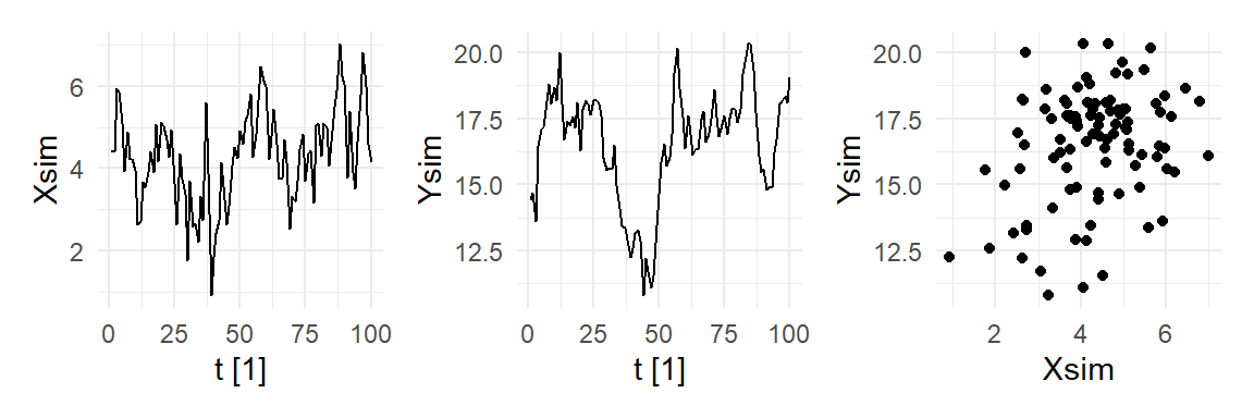
We see that the usual standard errors lead to incorrect inferences. The heteroskedasticity-robust standard errors are similar to the usual standard errors, which is not surprising since there is in fact no heteroskedasticity in this data set. They also lead to incorrect inference on the coefficient of Xsim. The HAC standard errors are substantially larger, resulting in smaller t-statistics, and correct inference. The HAC standard errors are appropriate as \(X_{t}\epsilon_{t}\) is correlated (see Fig. 11.23)
ACF(df, Xsim*residuals(mdlsim)) %>% autoplot() + theme_minimal()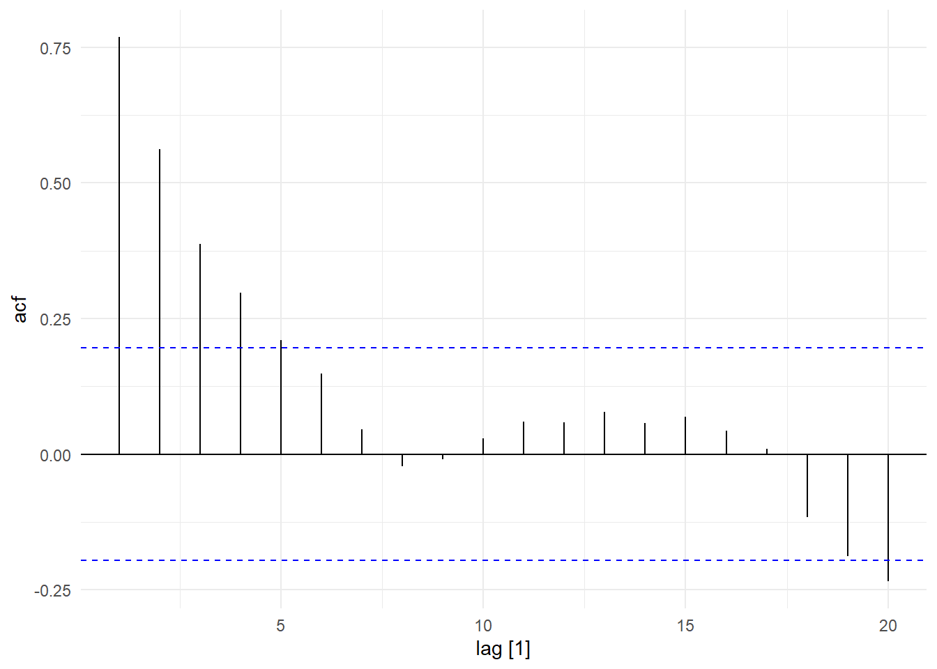
11.3.4 Dynamically Complete Models
Often we try to ensure that our time series models are dynamically complete, i.e., that sufficient number of lags of the dependent and independent variables are included so that there are no dynamics left in the noise term. One reason for this is if the model is being built for forecasting purposes. In that case we want to ensure that the full dynamic properties of the time series is accounted for by the model. Another reason is that sometimes we want to include lagged dependent variables in the specification, and the presence of both lagged dependent variables and serial correlation may lead to inconsistent estimators. For instance, suppose \[ Y_{t} = \alpha_0 + \alpha_1 Y_{t-1} + u_{t} \] with \(|\alpha_1|<0\) and where \(u_{t} = \epsilon_{t} + \theta \epsilon_{t-1}\), \(\epsilon_{t} \sim_{iid} (0,\sigma^2)\). Then the error term \(u_{t}\) is correlated with \(Y_{t-1}\) (see exercises for details). This means that contemporaneous exogeneity does not hold, resulting in inconsistent OLS estimators.
11.3.5 Testing for Autocorrelation
To check for autocorrelation in a regression, it is common practice to plot the sample acf of the residuals, i.e., after running the regression \[ Y_{t} = x_{t}^\mathrm{T}\beta + \epsilon_{t} \] we collect the residuals \(\hat{\epsilon}_{t}\) and compute its sample acf. This often gives us a good indication of the presence of serial correlation in the errors.
To more formally test for autocorrelation, one can run a regression of \(\hat{\epsilon}_t\) on lags of \(\hat{\epsilon}_t\), and on the regressors, i.e., regress \[ \hat{\epsilon}_t \text{ on } \hat{\epsilon}_{t-1}, \dots, \hat{\epsilon}_{t-p}, x_{1,t}, \dots, x_{K-1,t} \] where \(x_{1,t},\dots,x_{K-1,t}\) are the regressors in \(x_t^\mathrm{T}\). Then test for the significance of the coefficients on the lagged residuals.
11.3.6 Regression with Trending and Persistent Series
If there is trend or seasonality in the time series in the regression, these must be accounted for. In the following example, we regress log(ELEC_GEN_SG) on log(IP_SG) twice, once without seasonals or trend, and another time with both. That is, we run the regressions \[ Y_{t} = \alpha_0 + \beta_0X_{t} + \epsilon_{t} \tag{11.19}\] and \[ Y_{t} = \alpha_0 + \beta_0X_{t} + seas.\;dummies + \delta_1 t + \delta_2 t^2 + \epsilon_{t} \tag{11.20}\]
ts03 <- readxl::read_excel("data\\ts_01.xlsx") %>%
        select(DATE, IP_SG, ELEC_GEN_SG) %>%
        mutate(DATE=yearmonth(DATE)) %>%
        as_tsibble(index=DATE)
## We use the TSLM() function in fpp3 which allows us to include seasonal dummies
## and trend simply by including season() and trend() in the regression formula
mdl_elec1 <- ts03 %>% model(TSLM(log(ELEC_GEN_SG)~log(IP_SG)))
report(mdl_elec1)
Series: ELEC_GEN_SG
Model: TSLM
Transformation: log(ELEC_GEN_SG)
Residuals:
Min 1Q Median 3Q Max
-0.23353 -0.06955 -0.01108 0.06348 0.28123
Coefficients:
Estimate Std. Error t value Pr(>|t|)
(Intercept) 4.510243 0.028988 155.6 <2e-16 ***
log(IP_SG) 0.836081 0.007494 111.6 <2e-16 ***
---
Signif. codes: 0 '***' 0.001 '**' 0.01 '*' 0.05 '.' 0.1 ' ' 1
Residual standard error: 0.101 on 418 degrees of freedom
Multiple R-squared: 0.9675, Adjusted R-squared: 0.9674
F-statistic: 1.245e+04 on 1 and 418 DF, p-value: < 2.22e-16mdl_elec2 <- ts03 %>% model(TSLM(log(ELEC_GEN_SG)~log(IP_SG)+season()+trend()+I(trend()^2)))
report(mdl_elec2)Series: ELEC_GEN_SG
Model: TSLM
Transformation: log(ELEC_GEN_SG)
Residuals:
Min 1Q Median 3Q Max
-0.095765 -0.019684 -0.003458 0.021550 0.101889
Coefficients:
Estimate Std. Error t value Pr(>|t|)
(Intercept) 6.235e+00 4.290e-02 145.325 < 2e-16 ***
log(IP_SG) 8.882e-02 1.701e-02 5.221 2.85e-07 ***
season()year2 -8.801e-02 7.592e-03 -11.593 < 2e-16 ***
season()year3 3.301e-02 7.640e-03 4.321 1.96e-05 ***
season()year4 2.397e-02 7.394e-03 3.242 0.00128 **
season()year5 6.398e-02 7.394e-03 8.654 < 2e-16 ***
season()year6 3.126e-02 7.430e-03 4.207 3.19e-05 ***
season()year7 5.519e-02 7.418e-03 7.441 6.04e-13 ***
season()year8 4.575e-02 7.434e-03 6.153 1.82e-09 ***
season()year9 1.455e-02 7.528e-03 1.933 0.05389 .
season()year10 4.584e-02 7.464e-03 6.142 1.95e-09 ***
season()year11 -9.464e-04 7.396e-03 -0.128 0.89824
season()year12 -3.467e-03 7.525e-03 -0.461 0.64524
trend() 7.748e-03 1.413e-04 54.846 < 2e-16 ***
I(trend()^2) -8.901e-06 1.517e-07 -58.661 < 2e-16 ***
---
Signif. codes: 0 '***' 0.001 '**' 0.01 '*' 0.05 '.' 0.1 ' ' 1
Residual standard error: 0.03093 on 405 degrees of freedom
Multiple R-squared: 0.997, Adjusted R-squared: 0.9969
F-statistic: 9768 on 14 and 405 DF, p-value: < 2.22e-16The log(IP_SG) variable is significant in both regressions, but its estimated coefficient in the regression with trend and seasonal dummies is one-tenth of that in the regression without trend and seasonality. Notice that the \(R^2\) is very high. This is usually the case in regressions with trend.
The model is dynamically incomplete. There is autocorrelation in the error terms, as can be seen from the ACF of the residuals, reported in Fig. 11.24 below.
p1 <- autoplot(residuals(mdl_elec2), .resid) + theme_minimal()
p2 <- ACF(residuals(mdl_elec2), .resid) %>% autoplot() + theme_minimal()
(p1 | p2) + plot_annotation(tag_levels = 'a')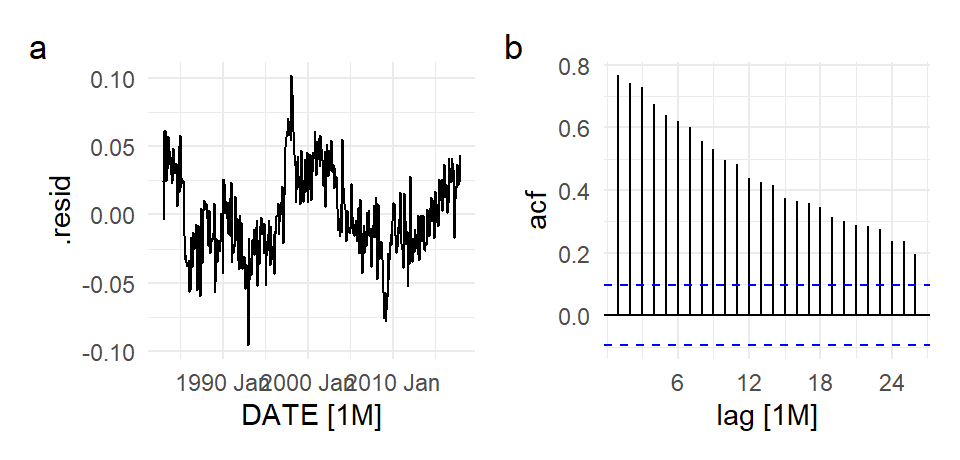
We add three lags of log(ELEC_GEN_SG) in the next model, i.e., we fit the model \[ \begin{aligned} Y_{t} = \alpha_0 + \beta_0X_{t} &+ \gamma_1Y_{t-1} + \gamma_2Y_{t-2} + \gamma_3Y_{t-3} \\ &+ seas.\;dummies + \delta_1 t + \delta_2 t^2 + \epsilon_{t} \end{aligned} \tag{11.21}\] Fig. 11.25 shows the fit (in terms of ELEC_GEN_SG, not log(ELEC_GEN_SG)), the residuals, and the ACF of the residuals.
mdl_elec3 <- ts03 %>% model(TSLM(log(ELEC_GEN_SG)~
                                   log(IP_SG) +
                                   lag(log(ELEC_GEN_SG),1)+
                                   lag(log(ELEC_GEN_SG),2)+
                                   lag(log(ELEC_GEN_SG),3)+
                                   season()+trend()+I(trend()^2)))
report(mdl_elec3)
Series: ELEC_GEN_SG
Model: TSLM
Transformation: log(ELEC_GEN_SG)
Residuals:
Min 1Q Median 3Q Max
-0.0600626 -0.0101659 -0.0001068 0.0115216 0.0646623
Coefficients:
Estimate Std. Error t value Pr(>|t|)
(Intercept) 7.281e-01 2.029e-01 3.588 0.000375 ***
log(IP_SG) 5.900e-02 1.015e-02 5.810 1.28e-08 ***
lag(log(ELEC_GEN_SG), 1) 3.427e-01 4.624e-02 7.411 7.56e-13 ***
lag(log(ELEC_GEN_SG), 2) 2.662e-01 4.697e-02 5.668 2.77e-08 ***
lag(log(ELEC_GEN_SG), 3) 2.553e-01 4.609e-02 5.539 5.53e-08 ***
season()year2 -7.666e-02 5.145e-03 -14.901 < 2e-16 ***
season()year3 8.175e-02 6.241e-03 13.099 < 2e-16 ***
season()year4 4.937e-02 7.095e-03 6.958 1.42e-11 ***
season()year5 8.335e-02 9.303e-03 8.959 < 2e-16 ***
season()year6 7.674e-03 5.207e-03 1.474 0.141365
season()year7 3.547e-02 5.743e-03 6.175 1.63e-09 ***
season()year8 1.584e-02 4.830e-03 3.280 0.001130 **
season()year9 -1.017e-02 5.507e-03 -1.847 0.065446 .
season()year10 2.630e-02 4.825e-03 5.450 8.83e-08 ***
season()year11 -2.249e-02 4.846e-03 -4.641 4.72e-06 ***
season()year12 -5.814e-03 5.513e-03 -1.055 0.292223
trend() 6.625e-04 2.737e-04 2.421 0.015939 *
I(trend()^2) -9.391e-07 3.067e-07 -3.062 0.002346 **
---
Signif. codes: 0 '***' 0.001 '**' 0.01 '*' 0.05 '.' 0.1 ' ' 1
Residual standard error: 0.01825 on 399 degrees of freedom
Multiple R-squared: 0.999, Adjusted R-squared: 0.9989
F-statistic: 2.237e+04 on 17 and 399 DF, p-value: < 2.22e-16p0 <- autoplot(ts03, ELEC_GEN_SG, color="blue") +
autolayer(fitted(mdl_elec3),.fitted, color="green") +
theme_minimal()
p1 <- autoplot(residuals(mdl_elec3), .resid) + theme_minimal()
p2 <- ACF(residuals(mdl_elec3), .resid) %>%
autoplot() + theme_minimal() + ylim(c(-1,1))
p0 / (p1 | p2) + plot_annotation(tag_levels = 'a')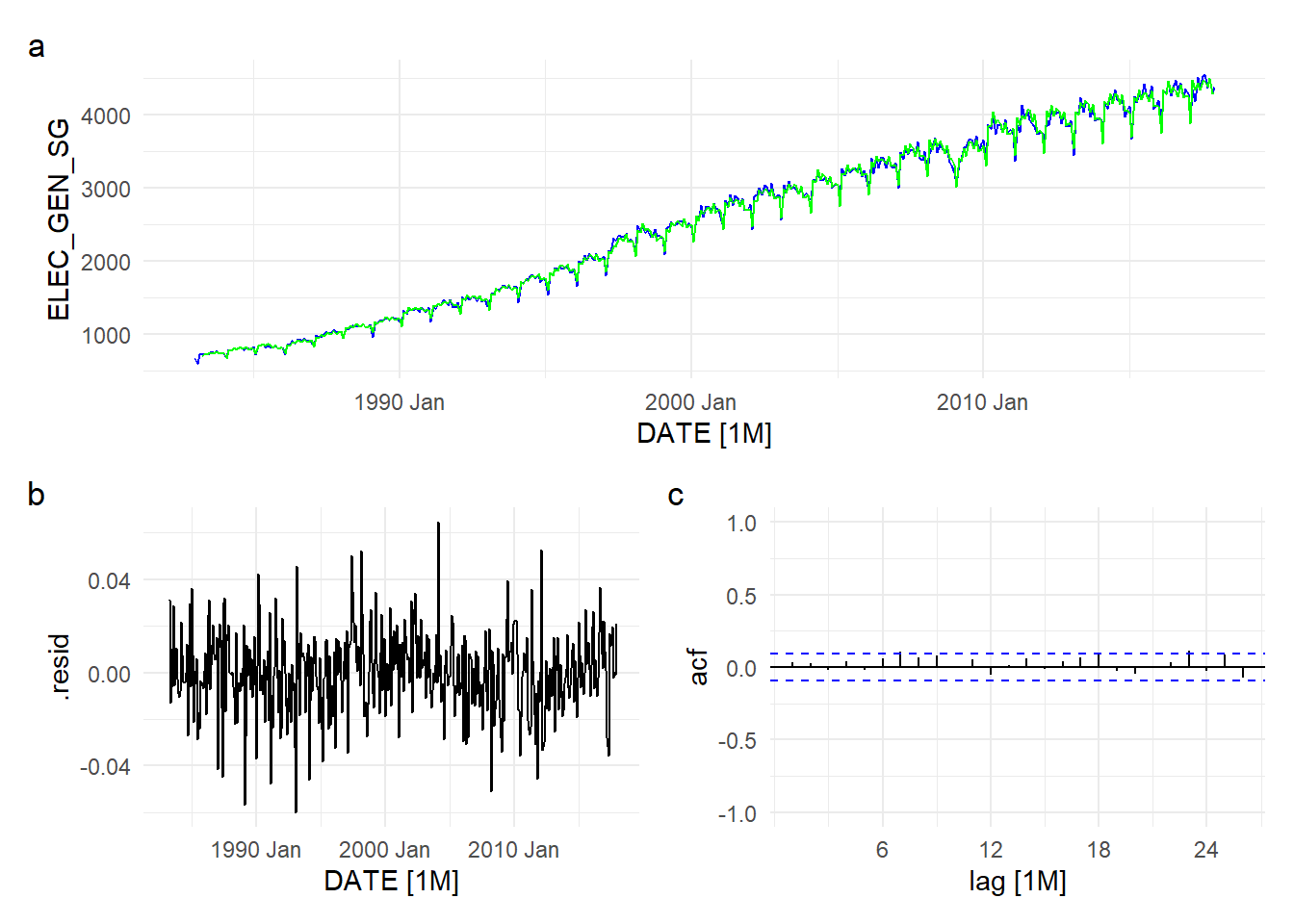
11.3.7 Spurious Regressions
We run another experiment as an illustration of what can go wrong if one is not working with weakly dependent data. We simulate \(200\) pairs of unrelated series \((X_{t}^{(r)},Y_{t}^{(r)})_{t=1}^{100}\), \(r=1,2,...,R\) as random walks: \[ \begin{aligned} X_{t}^{(r)} &= \alpha_{X} + X_{t-1}^{(r)} + u_{t}^{(r)} \\ Y_{t}^{(r)} &= \alpha_{Y} + Y_{t-1}^{(r)} + v_{t}^{(r)} \end{aligned} \] where \(u_{t}^{(r)}\) and \(v_{t}^{(r)}\) are independent \(\text{Normal}(0,1)\) noise terms. We set \(\alpha_{X}=0.5\) and \(\alpha_{Y}=0.8\). As explained earlier, these are trending series. For each replication \(r\), we regress \(Y_{t}^{(r)}\) on \(X_{t}^{(r)}\), with intercept, and collect the t-statistic on the coefficient of \(X_{t}^{(r)}\). We replicate this experiment 200 times. The histogram of the 200 t-statistics is shown in panel (a) below.
simRW <- function(a0, bigT){
  Z <- rep(0,bigT)
  u <- rnorm(bigT,0,1)
  for (t in 2:bigT){
    Z[t] <- a0 + Z[t-1] + u[t]
  }
  return(Z)
}
simExp <- function(R,bigT,aX,aY){
tstats <- rep(NA,R)
for (r in 1:R){
  X <- simRW(aX,bigT)
  Y <- simRW(aY,bigT)
  df <- data.frame(X,Y)
  mdl <- lm(Y~X, data=df)
  tstats[r] <- summary(mdl)$coefficients[2,'t value']
  }
return(tstats)
}
set.seed(13);
tstats1 <- simExp(200,100,0.4,0.8)
df <- data.frame(tstats1)
ggplot(df, aes(x=tstats1)) +
  geom_histogram(binwidth=3, color="black",fill="grey") + theme_minimal()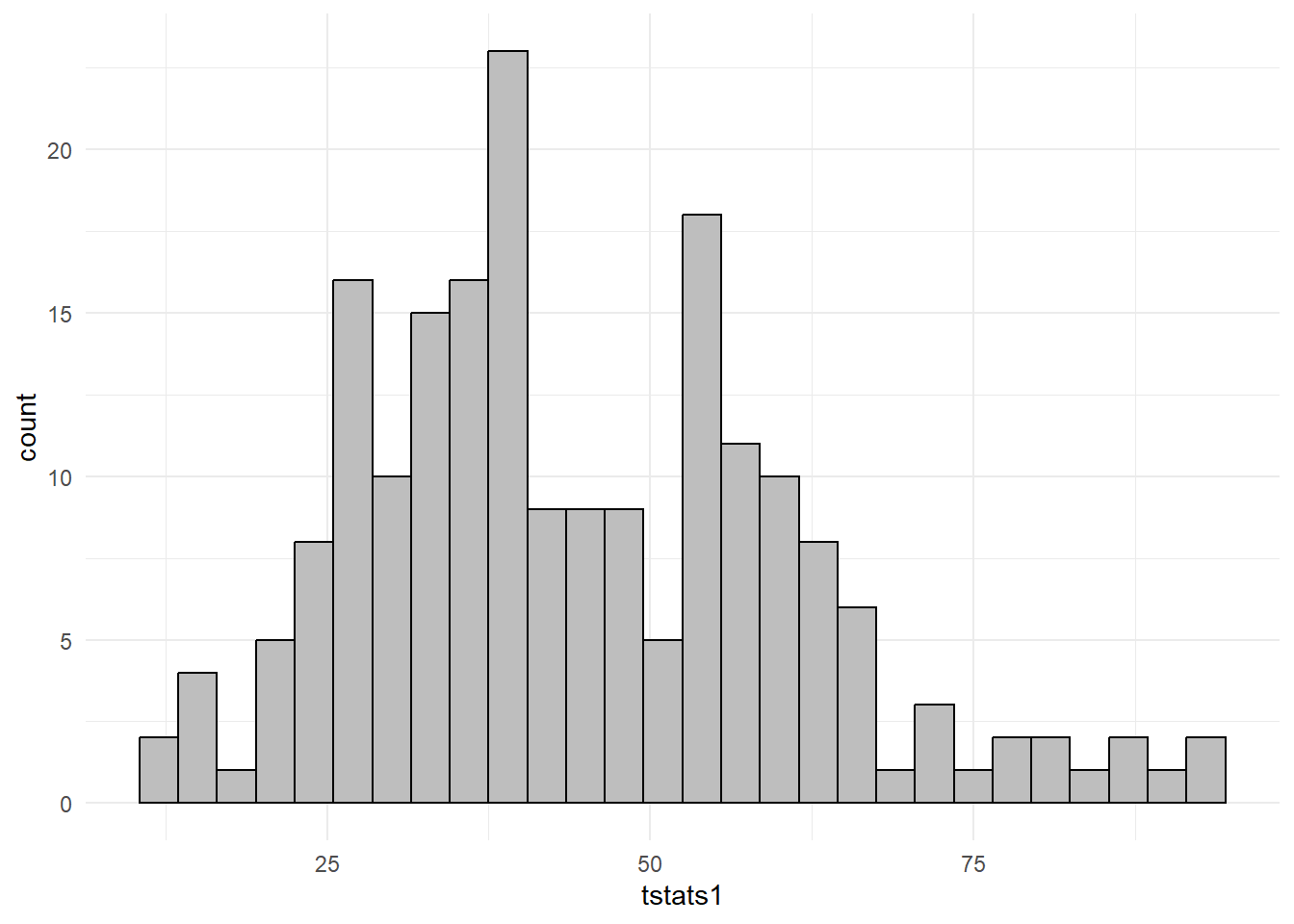
Because \(X_{t}^{(r)}\) and \(Y_{t}^{(r)}\) are completely unrelated, one might expect the estimate of the \(X_{t}^{(r)}\) coefficient to be statistically insignificant. However, the histogram in Fig. 11.26 above shows that all of the t-statistics over our 200 replications are greater than 2. Given that the two series are trending, this is not too surprising. Fig. 11.27 shows the time series plots of one such pair (panels a and b), together with their scatterplot (panel c). It is clear that the linear regression of \(Y_{t}^{(r)}\) on \(X_{t}^{(r)}\) is merely capturing the fact that both series are increasing over time.
set.seed(13)
X <- simRW(0.4,100)
Y <- simRW(0.8,100)
dfplot <- data.frame(t=1:100,X,Y)
p1 <- dfplot %>% ggplot() + geom_point(aes(x=t,y=X)) + theme_minimal()
p2 <- dfplot %>% ggplot() + geom_point(aes(x=t,y=Y)) + theme_minimal()
p3 <- dfplot %>% ggplot() + geom_point(aes(x=X,y=Y)) + theme_minimal()
(p1 | p2 | p3) + plot_annotation(tag_levels = "a")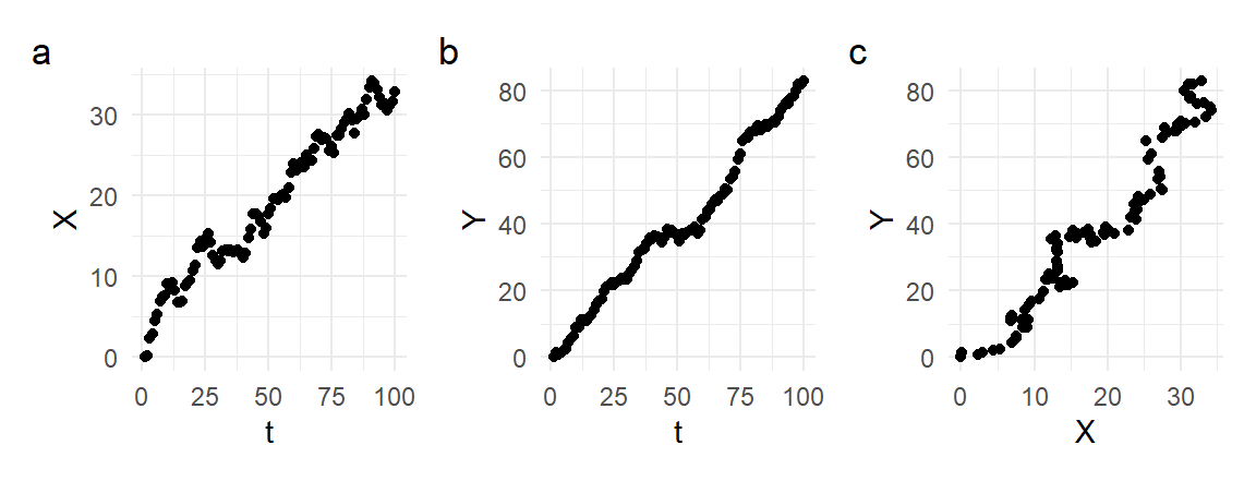
The interesting thing about this result is that it persists even if \(\alpha_{X}\) and \(\alpha_{Y}\) are both set to zero, i.e., if \[ \begin{aligned} X_{t}^{(r)} &= X_{t-1}^{(r)} + u_{t}^{(r)} \\ Y_{t}^{(r)} &= Y_{t-1}^{(r)} + v_{t}^{(r)} \end{aligned} \] so that there are no drifts in the series. Repeating the experiment with this change, we obtain the following t-statistic histogram over 200 replications.
set.seed(13);
tstats2 <- simExp(200,100,0,0)
df <- data.frame(tstats2)
ggplot(df, aes(x=tstats2)) +
  geom_histogram(binwidth=2, color="black",fill="grey") + theme_minimal()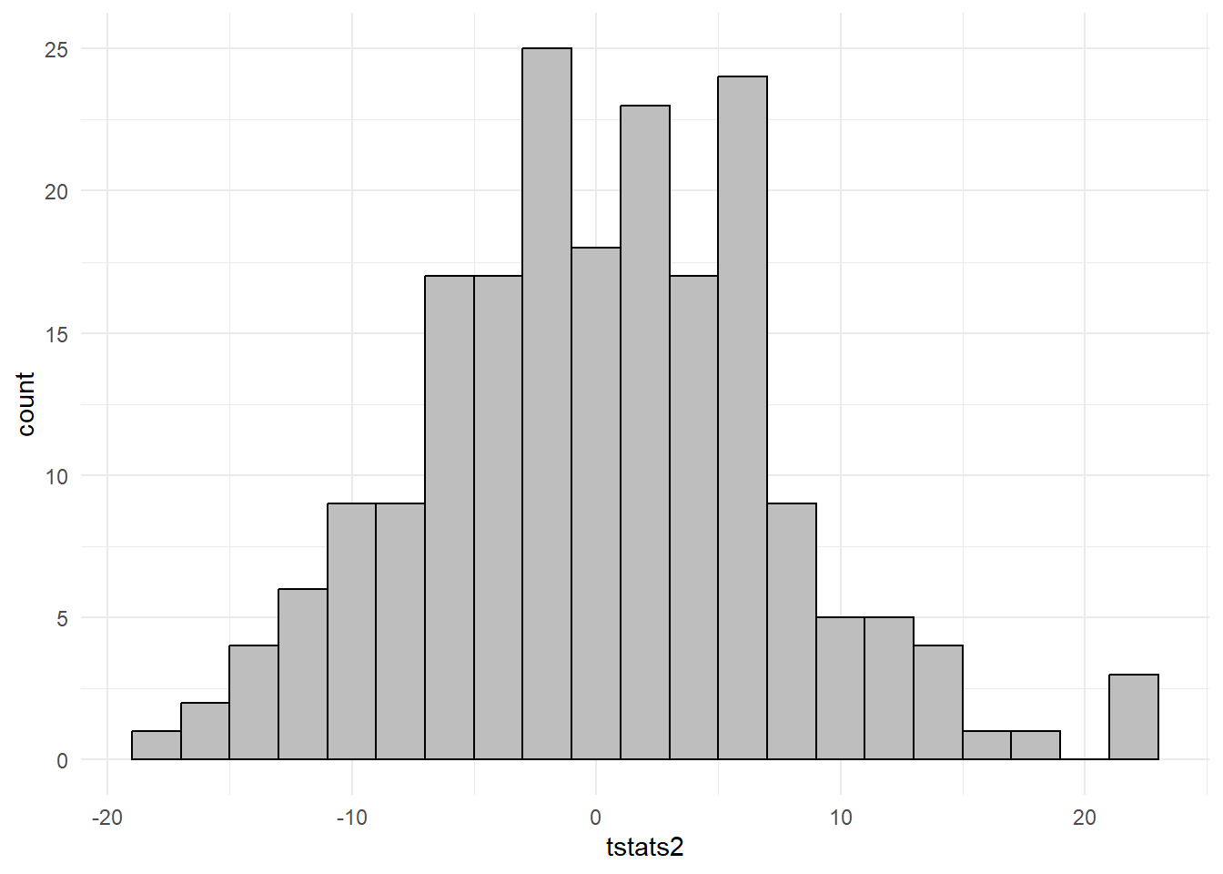
We find that in the vast majority (about 80%) of the replications, the t-statistic is greater than two, well in excess of 5%. This result is known as “spurious regressions”, and we leave a fuller discussion of this issue for a later chapter.
11.4 Exercises
Exercise 11.1
- Show that the first-order Taylor (i.e., linear) approximation to the (natural) log function leads to the approximation \[ \frac{Y_{t} - Y_{t-1}}{Y_{t-1}} \approx \ln Y_{t} - \ln Y_{t-1}\,. \]
- Show that \(\ln Y_{t} - \ln Y_{t-1}\) can also be viewed as the (exact) continuous growth rate over period \(t\) (assume that measurements of \(Y\) are taken at the end of each period).
Exercise 11.2 A popular transformation to apply to time series data is the Box-Cox transformation \[ y(\lambda)=\begin{cases} \dfrac{y^\lambda-1}{\lambda} & \text{ if } \;\lambda \neq 0 \\ \ln(y) & \text{ if } \;\lambda=0\ \end{cases} \] for some given \(\lambda\). This transformation is only used when \(y>0\). Show that \[ \dfrac{y^\lambda-1}{\lambda} \rightarrow \ln(y) \quad \text{as} \quad \lambda \rightarrow 0\,. \]
Exercise 11.3 The monthly seasonal dummy specification \[ Y_{t} = \delta_{0} + \delta_{2}(d_{2,t}-\tfrac{1}{12})+\delta_{3}(d_{3,t}-\tfrac{1}{12}) + \dots + \delta_{12}(d_{12,t}-\tfrac{1}{12}) + \epsilon_{t}. \tag{11.22}\] produces an equivalent fit to the specifications (11.4) and (11.5). Find interpretations for the parameters \(\delta_{0}, \delta_{2}, \dots, \delta_{12}\).
Exercise 11.4 How would you test for the presence of seasonality using the seasonal dummy models (11.4), (11.5) and (11.22)? State the exact hypotheses to be tested.
Exercise 11.5 Suppose the price of a certain product is determined by supply and demand as specified below: \[ \begin{aligned} Q_{t}^{s} &= \alpha_{0} + \alpha_{1} P_{t} + \alpha_{2} P_{t-1}+\epsilon_{t}^{s} &(\text{supply equation}) \\ Q_{t}^{d} &= \delta_{0} + \delta_{1} P_{t}+ \epsilon_{t}^{d} &(\text{demand equation}) \\ Q_{t}^{s} &= Q_{t}^{d} &(\text{market clearing}) \end{aligned} \] where the demand and supply shocks \(\epsilon_{t}^{s}\) and \(\epsilon_{t}^{d}\) are zero-mean independent noise term. Show that price \(P_{t}\) follows an AR(1) process by equating the supply and demand equations and solving for \(P_{t}\) in terms of \(P_{t-1}\) and the demand and supply shocks.
Exercise 11.6 Re-parameterize the distributed lag model \[ Y_{t} = \alpha_0 + \beta_0X_t + \beta_1X_{t-1} + \beta_2X_{t-2} + \epsilon_t \] so that the long-run cumulative dynamic multiplier \(\beta_0 + \beta_1 + \beta_2\) appears as a coefficient on a regressor. Remark: Estimating a version where the long-run cumulative dynamic multiplier is a coefficient on a regressor makes it much easier to obtain the standard errors on the sum \(\hat{\beta}_0+\hat{\beta}_1+\hat{\beta}_2\).
Exercise 11.7 Suppose \[ Y_{t} = \alpha_0 + \alpha_1 Y_{t-1} + u_{t} \] with \(|\alpha_1|<1\) and where \(u_{t} = \epsilon_{t} + \theta \epsilon_{t-1}\), \(\epsilon_{t} \sim_{iid} (0,\sigma^2)\). In this exercise we will show that \(Y_{t-1}\) and \(u_{t}\) are correlated, so that even contemporaneous exogeneity does not hold.
Show that \(\mathrm{E}[u_{t} u_{t-1}] = \theta \sigma^2\).
Show that \(\mathrm{E}[u_{t} u_{t-j}] = 0\) for all \(j > 1\).
Show that \(Y_{t}\) can be written as \[ Y_{t} = \frac{\alpha_{0}}{1-\alpha_{1}} + u_{t} + \alpha_{1} u_{t-1} + \alpha_{1}^2 u_{t-2} + \dots \]
Show that \(\mathrm{E}[u_{t} Y_{t-1}] = \theta \sigma^2\).
Exercise 11.8 When we fit (11.20) on the log(ELEC_GEN_SG) series we obtained a very high \(R^2\). This is often the case when fitting models with trend to models. Much of the explanatory power may be coming from the trend component. Run a regression of log(ELEC_GEN_SG) on the seasonal dummies and the quadratic trend and collect the residuals. Do the same with log(IP_SG). Now run a regression of the residuals from the log(ELEC_GEN_SG) regression on to the residuals from the log(IP_SG) regression. Confirm that the coefficient on the log(IP_SG) residuals are the same as the coefficient on log(IP_SG) in (11.20). What is the \(R^2\) from the residual regression?
11.5 Appendix
There are methods that measure trend without requiring a decision on the form of the trend. The Hodrick-Prescott (HP) filter, popular among macroeconomists, is one such method. Denoting the trend as \(\tau_{t}\), the method chooses \(\hat{\tau_{t}}\), \(t=1,2,...,T\) to minimize the sum of squared residuals \(\sum_{t=1}^{T}(y_{t}-\hat{\tau}_{t})^2\), while controlling for the overall level of “wigglyness” of the estimated trend. Specifically, the HP method sets: \[ {\hat{\tau}_{t}^{hp}} = \mathrm{argmin}_{\hat{\tau}_{t}} \left(\sum_{t=1}^{T}(y_{t}-\hat{\tau}_{t})^2 + \lambda \sum_{t=2}^{T-1}\left[(\hat{\tau}_{t+1}-\hat{\tau}_{t}) - (\hat{\tau}_{t}-\hat{\tau}_{t-1}) \right]^2 \right) \tag{11.23}\] for some given value of \(\lambda>0\). The first term in the minimization is the sum of squared residuals. In the second summation, \(\hat{\tau}_{t} - \hat{\tau}_{t-1}\) is the change in the estimated trend from \(t-1\) to \(t\), and \(\hat{\tau}_{t+1} - \hat{\tau}_{t}\) is the change from period \(t\) to \(t+1\). The term \[ \sum_{t=2}^{T-1}\left[(\hat{\tau}_{t+1}-\hat{\tau}_{t}) - (\hat{\tau}_{t}-\hat{\tau}_{t-1}) \right]^2 \] is therefore a measure of how quickly \(\hat{\tau}_{t}\) is change at \(t=2,3,...,T-1\), analogous to a second derivative. The second derivative measures how quickly a slope is changing – a large absolute second-derivative at a certain point indicates that the slope is changing very quickly at the point, i.e., the function is bending very sharply at that point. In the case of a straight time, the second derivative is zero everywhere.
We can get a sense of the HP filter works by imagining extreme values of \(\lambda\). Setting \(\lambda=0\), the second term becomes irrelevant, and we can minimize (11.23) by setting \(\hat{\tau}_{t}^{hp}=y_{t}\) for all \(t\). In other words, we simply connect the dots. Setting \(\lambda=\infty\), the slightest bend in the proposed trend results in (11.23) becoming infinity, so minimization is achieved by fitting a straight line through the data.
The following is an application to the log(IP_SG) with \(\lambda=129600\), the value of \(\lambda\) that has been recommended for monthly data. There series in Fig. 11.29(b) is the detrended log(IP_SG) after the HP trend is removed.
ts03.ts <- as.ts(ts03)
lipsg <- mFilter::hpfilter(log(ts03.ts[,'IP_SG']), type="lambda", freq=129600)
hp_dat <- as_tsibble(ts.union("hpcycle"=lipsg$cycle,
                   "hptrend"=lipsg$trend,
                   "log(IP_SG)"=log(ts03.ts[,'IP_SG'])),pivot_longer=F)
p1 <- autoplot(hp_dat, `log(IP_SG)`, color="grey") +
      autolayer(hp_dat, hptrend, size=0.8) +
      theme_minimal() + theme(legend.position = "bottom")
p2 <- autoplot(hp_dat, hpcycle) + theme_minimal()
(p1 | p2) + plot_annotation(tag_levels = 'a')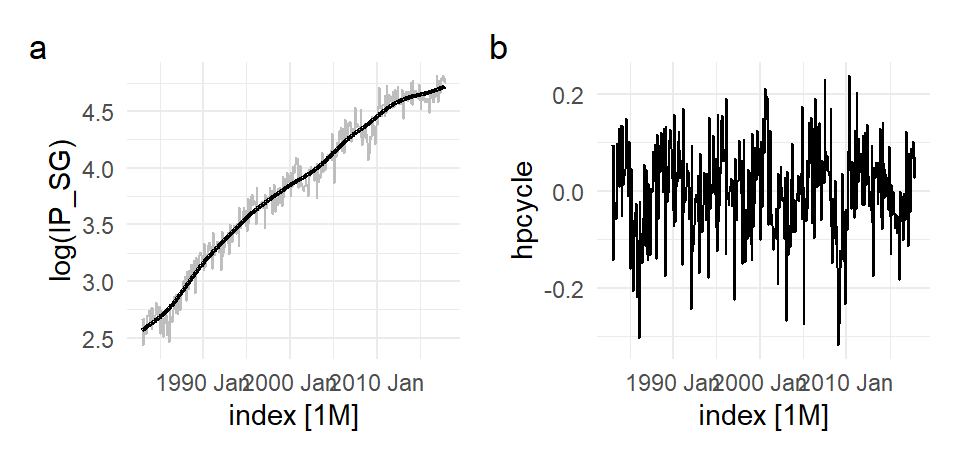
One difficulty with trend fitting and de-trending is that what remains (cycles, seasonalities, and other features) depends on what is taken out. It is sometimes difficult to tell what is trend (“long-term” movements) and what is cycle (“medium term” movements?). Repeating the exercise above with \(\lambda=1600\) (the value usually recommended for quarterly data, even though we have monthly data) gives:
## uses mFilter package
lipsg <- mFilter::hpfilter(log(ts03.ts[,'IP_SG']), type="lambda", freq=1600)
hp_dat <- as_tsibble(ts.union("hpcycle"=lipsg$cycle,
                   "hptrend"=lipsg$trend,
                   "log(IP_SG)"=log(ts03.ts[,'IP_SG'])),pivot_longer=F)
p1 <- autoplot(hp_dat, `log(IP_SG)`, color="grey") +
      autolayer(hp_dat, hptrend, size=0.8) +
      theme_minimal() + theme(legend.position = "bottom")
p2 <- autoplot(hp_dat, hpcycle) + theme_minimal()
(p1 | p2) + plot_annotation(tag_levels = 'a')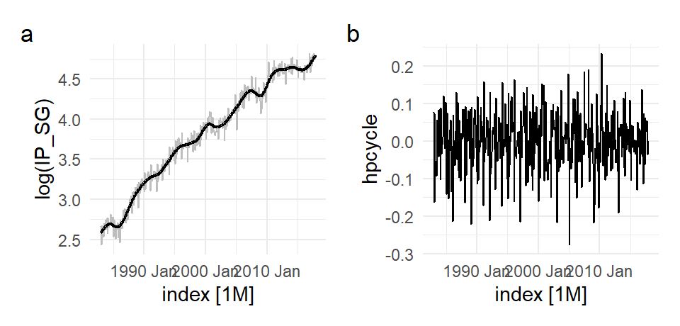
The fitted trend fluctuates substantially more, and one suspects that it has picked up more than just trend. The fitted line here might be better thought of as “trend and cycle”.
The HP filter is an example of a non-parametric technique. Another much more elementary non-parametric approach is to use a “moving-average”: \[ \hat{\tau}_{t}^{ma} = \frac{1}{2k+1}\sum_{j=-k}^{k}Y_{t+j} , t=k+1,..., T-k \] for some chosen bandwidth \(k\). Note that the specific version of the technique shown here does not provide estimates on either end of the series (there are versions that do). The “local” nature of this method means that the results should be considered “trend and cycle” unless a very large \(k\) is chosen, but then that would only provide estimates for a small portion of the data. The following smooths the log(IP_SG) series with \(k=10\)
ma_dat <- ts03 %>% mutate("MA"=as.numeric(NA))
k <- 10
T <- dim(ma_dat)[1]
ma_dat[(k+1):(T-k),"MA"] <- zoo::rollmean(log(ma_dat[,"IP_SG"]), 2*k+1, align="center")
autoplot(ma_dat, log(IP_SG), color="darkgray") +
      autolayer(ma_dat, MA, size=0.8) + theme_minimal() +
      theme(legend.position = "bottom")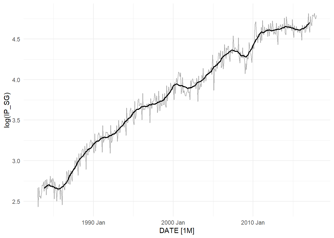
Decompositions can be “additive” or “multiplicative”. In this case it is additive, and the seasonally-adjusted series is obtained by substracting the seasonal component from the original.↩︎
There are formal ways to define “weakly dependent”, but we will make do with our informal characterization for now.↩︎