4 Statistics Review

Many problems in statistics involve estimating the population mean of a variable and testing hypotheses regarding its value. Often the sample average of the observations are used as an estimate of the population mean. We do so because we know a priori that in many circumstances the sample mean is a good estimator (i.e., a good estimation rule) for the population mean.

In this chapter, we review the ideas behind parameter estimation and hypothesis testing using the example of estimating and testing a population mean, including an extended discussion of what “good” means in the context of parameter estimation. We then go through in detail a simple application to illustrate the theory. The R code in this chapter uses the tidyverse and patchwork packages.

library(tidyverse)
library(patchwork)

4.1 Estimation

Suppose $Y$ is a random variable with mean $\mu$ and variance $\sigma^{2}$. You are interested in

estimating $\mu$,
getting some idea how “good” (accurate, precise, etc.) your estimate is,
testing if $\mu$ is equal to some hypothesized value $\mu_0$, i.e., checking to see if you have statistical evidence to reject $\mu = \mu_{0}$.

Suppose you will be able to obtain a random sample of $N$ observations $Y_{1}$, $Y_{2}$, …, $Y_{N}$ of this variable, but suppose you haven’t yet obtained this sample, so for the moment, $Y_{1}$, $Y_{2}$, …, $Y_{N}$ are all random variables. We will nonetheless continue to refer to them as the sample. The term “random sample” means that your sample are i.i.d. random variables of $X$, so they are all uncorrelated with each other, and $E[Y_{i}]=\mu$ and $var[Y_{i}] = \sigma^2$ for all $i$.

4.1.1 Unbiased Estimators

Since you are estimating a population mean, suppose you propose to use the sample mean \[ \hat{\mu} = \frac{1}{N}\sum_{i=1}^{N} Y_{i} = \overline{Y} \tag{4.1}\] as an estimator for $\mu$.

We will switch between the notation $\hat{\mu}$ and $\overline{Y}$, using the former especially when we want to highlight the fact that we are estimating the population mean. Take note to distinguish between the population mean and the sample mean. The population mean is the constant $E[Y]=\mu$. The sample mean is the expression in Eq. 4.1, which because it is made of random variables, is itself a random variable. You are proposing to use the sample mean as an estimator for the population mean. When you do finally collect your sample realizations, you will plug in those realizations into Eq. 4.1 to calculate your estimate of the population mean. An estimate (an actual number) is a realization of the estimator (a random variable).

Is your proposal to use the sample mean as an estimator for the population mean a good one? First, what is your criteria for deciding what makes a good estimator?

One criterion used is unbiasedness. The estimator $\hat{\theta}$ is said to be unbiased for $\theta$ if \[ E[\hat{\theta}] = \theta\,. \] That is, the distribution of your estimator is centered about the population mean. You can interpret this to mean that by following the estimation rule $\hat{\theta}$ you will not be systematically over- or under-estimating your target parameter.

Theorem 4.1 Suppose you have an i.i.d. sample $Y_{1}$, $Y_{2}$, …, $Y_{N}$ of a random variable $Y$ with mean $E[Y] = \mu$ and variance $var[Y] = \sigma^{2}$. Then \[ E[\overline{Y}] = E \left[ \frac{1}{N}\sum_{i=1}^N Y_i \right] = \frac{1}{N}\sum_{i=1}^N E[Y_i] = \frac{1}{N} N \mu = \mu \tag{4.2}\] and \[ var[\overline{Y}] = var \left[ \frac{1}{N}\sum_{i=1}^N Y_i \right] = \frac{1}{N^{2}}\sum_{i=1}^N var[Y_i] = \frac{1}{N^2} N \sigma^{2} = \frac{\sigma^{2}}{N}\,. \tag{4.3}\]

Eq. 4.2 says that the sample mean is an unbiased estimator for the population mean. Theorem 4.1 also provides an expression for the variance of the sample mean. For the variance, we made use of the “independence” assumption, so the sample is an uncorrelated sample, and the variance of the sum became the sum of the variance. Note that for the unbiasedness part, we did not require uncorrelated samples.

Example 4.1 (An example of a biased estimator) We should always provide an estimate of the variance (or standard error) of our estimator.¹ For the sample mean, this requires estimating $\sigma^2 = var[Y]$, and using this estimate in Eq. 4.3. Since $var[Y]=E[(Y-E[Y])^2] = E[Y^2] - E[Y]^2$, it seems reasonable to consider estimating $\sigma^2$ with

\[ \widetilde{\sigma^2} = \frac{1}{N}\sum_{i=1}^N (Y_i - \overline{Y})^2 = \frac{1}{N}\sum_{i=1}^N Y_i^2 - \overline{Y}^2 \,. \tag{4.4}\] However, this is a biased estimator for $\sigma^2$. Using $E[Y_i^2] = var[Y_i] + E[Y_i]^2 = \sigma^2 + \mu^2$ and $E[\overline{Y}^2] = var[\overline{Y}] + E[\overline{Y}]^2 = \sigma^2/N + \mu^2$, we have \[ E[\widetilde{\sigma^2}] = \frac{1}{N}\sum_{i=1}^N E[Y_i^2] - E[\overline{Y}^2] = \sigma^2 + \mu^2 - \frac{\sigma^2}{N}-\mu^2 = \frac{N-1}{N}\sigma^2. \] The estimator Eq. 4.4 therefore systematically under-estimates the variance of the sample observations. If your sample size $N$ is large, the bias may be negligible for all intents and purposes. Nonetheless, in this case it is easy to derive an unbiased estimator, namely \[ \widehat{\sigma^2} = \frac{N}{N-1}\widetilde{\sigma^2} = \frac{1}{N-1}\sum_{i=1}^N (Y_i - \overline{Y})^2. \tag{4.5}\] The intuition for why the divisor in Eq. 4.5 has to be $N-1$ instead of $N$ is that the deviations from sample mean always sum to zero. This means that there are only $N-1$ ‘free’ deviations from sample mean. For example, given $\sum_{i=1}^N (Y_i - \overline{Y})$ and the first $N-1$ deviations $(Y_i - \overline{Y})$, $i=1,2,...,N-1$, you can determine the $N$th deviation as $(Y_N - \overline{Y}) = - \sum_{i=1}^{N-1} (Y_i - \overline{Y})$. One “degree of freedom” was lost because we had to use the observations to compute the sample mean in order to compute the deviations from sample mean.

4.1.2 Efficiency

Unbiasedness is obviously a desirable property for an estimator, but on its own, it is hardly sufficient justification. After all, the estimator $\hat{\mu}_{1} = Y_{1}$, where you only pick the first observation and throw away the rest, is also unbiased: $E[\hat{\mu}_{1}] = E[Y_{1}] = \mu$. Of course we don’t want to use just one observation; the whole point of taking the average of several observations is so that positive and negative errors cancel out, leading to a better estimator.

The idea of positive and negative errors cancelling out is reflected in the variance of an estimator, which is a measure of how precise the estimator is. Since $var[\overline{Y}] = \frac{\sigma^2}{N}$, using all $N$ observations produces an estimator that is much more precise than using just a single observation, which gives a variance of $\sigma^{2}$. Even using just two observations reduces the estimator variance by half.

Obviously we want our sample size to be as large as possible. But we can in fact go further and claim that the sample mean, under the conditions we have stated, is the most precise among all “linear unbiased estimators”. In the context of statistical estimation, a linear estimator is one that takes the form $\sum_{i=1}^N a_iY_i$, and such an estimator will be unbiased if the $a_i$’s sum to one. The sample mean is a linear unbiased estimator² with $a_i = 1/N$ for $i=1,2,...,N$. It is the linear estimator with the smallest variance; we cannot tweak the weights to give us a more precise estimator.

The following argument proves that the sample mean has the smallest variance among all linear unbiased estimators. Suppose we have a linear unbiased estimator $\sum_{i=1}^N a_iY_i$ where $a_i \neq 1/N$ for at least one $i$. Write $a_i = 1/N + b_i$ where the $b_i$’s are not all zero, but sum to zero. This means that the estimator differs from the sample mean, but is nonetheless unbiased, since $\sum_{i=1}^N a_i=1$. Then \[ \begin{aligned} var[\widetilde{Y}] &= var\left[\sum_{i=1}^N \left(\frac{1}{N} + b_i \right)Y_i \right] \\ &= \sum_{i=1}^N \left(\frac{1}{N} + b_i \right)^2 var[Y_i] \\ &= var[\overline{Y}] + \sigma^2\sum_{i=1}^N b_i^2. \end{aligned} \tag{4.6}\] Since the $b_i$’s are not all zero, $\sum_{i=1}^N b_i^2 >0$, so $var[\widetilde{Y}] > var[\overline{Y}]$. We say that the sample mean is the most efficient among all linear unbiased estimators (we also say it is the ‘best linear unbiased’ estimator).

4.1.3 Mean Square Error

What we have done so far is taken a “lexicographical” approach to the criterion of unbiasedness and efficiency. We have justified the sample mean as being unbiased, and then argued that among all linear unbiased estimators, it is the most precise. Is there a criteria that combines both on an equal footing?

The mean square error (MSE) of an estimator $\hat{\theta}$ is defined as \[ MSE[\hat{\theta}] = E[(\hat{\theta} - \theta)^2]\,. \] The MSE can be decomposed into the estimator variance and square of the bias: \[ \begin{aligned} E[(\hat{\theta} - \theta)^2] &= var[\hat{\theta} - \theta] + E[(\hat{\theta} - \theta)]^2 \\ &= var[\hat{\theta}] + (E[\hat{\theta}] - \theta)^2] \\ &= var[\hat{\theta}] + bias^2 \end{aligned} \] where $bias = E[\hat{\theta}] - \theta$.

We might want an estimator that minimizes the MSE. Earlier, we found an estimator whose bias is zero, and then conditional on unbiasedness, minimum variance. Minimizing MSE considers both variance and bias simultaneously. In particular, we may find an estimator that is slightly biased, but has a much smaller variance, thereby reducing MSE. In other words, there may have a beneficial bias-variance trade-off.

It is easy to show that the sample mean minimizes the sample mean square error: suppose we choose $\hat{\mu}$ to minimize \[ \text{Sample MSE }= \sum_{i=1}^{N} (Y_{i} - \hat{\mu})^2\,. \] The first order condition is $-2\sum_{i=1}^{N} (Y_{i} - \hat{\mu})=0$ which you can solve for $\hat{\mu} = \overline{Y}$. The second derivative of the sample MSE with respect to $\hat{\mu}$ is $2>0$ so the sample mean solves the minimization problem. However, it does not necessarily minimize the population MSE $E[(\hat{\mu} - \mu)^2]$, and we may be able to find another estimator that produces a lower MSE.

We will see examples of this in the exercises.

4.2 A Coin Toss Example

How would we test if a coin is fair – that a random toss of the coin is as likely to show heads as it would tails? We could toss the coin a number of times and see if the frequency of heads is ‘reasonably’ close to half. How far from half should the frequency be for us to claim that the coin is not fair?

We can model the “experiment” of tossing the coin by describing the outcome as a random variable $Y$ with two possible values 0 and 1, where 0 indicates tails and 1 indicates heads, and where the probability of $Y=1$ is $p$ and the probability of $Y=0$ is $1-p$. Such a random variable is said to have a Bernoulli distribution, $Y \sim \mathrm{Bern}(p)$. The hypothesis that the coin is fair is $p=0.5$.

Suppose that each observation in our (as yet hypothetical) sample $\{Y_1,Y_2,...,Y_N\}$ is such that no one toss affects the outcome of any other, and that each of the $Y_i$ is Bernoulli with the same $p$. That is, we assume that the $Y_i$’s are independently and identically distributed with distribution $\mathrm{Bern}(p)$: \[ Y_i \overset{iid}{\sim} \mathrm{Bern}(p),i=1,2,..,N. \] When might a sample of coin tosses not be i.i.d.? Perhaps one lazily flips a coin back and forth, so we simply alternate between heads and tails (the observations are not uncorrelated). Or perhaps one (somehow) damages the coin during the flipping process, so that $p$ changes (observations are no longer identically distributed). Some individuals have been known to be skillful enough to willfully control the outcome of a coin toss. We rule out all such cases.

This application nicely fits our estimation theory of the previous section. We have an i.i.d. sample of observations of a random variable $Y$ with mean $p$. The only difference here is that there is not a separate parameter for the variance, which is $p(1-p)$. This does not cause any problems for us; we simply replace all instances of $\sigma^{2}$ with $p(1-p)$. Another difference is that we have more information in this example than in the previous section. In particular, we know the whole distribution of $Y$, whereas in the previous section we did not.

Since $p$ is the population mean of $Y$, we estimate it using the sample mean \[ \hat{p}=\overline{Y}. \] In this application, the sample mean is just the frequency of heads in the sample. From the theory discussed earlier we know that the sample mean is unbiased, and minimum variance among all linear unbiased estimators.

In fact, for this particular example the sample mean has the lowest variance among all unbiased estimators, linear or not. This is because the variance of the sample mean achieves a theoretical lower bound for unbiased estimators known as the Cramer-Rao Lower Bound. We omit a discussion of this for now.

The variance of $\hat{p} = \overline{Y}$ is $var[Y]/N$. Since $var[Y] = p(1-p)$, and $\hat{p}$ is an unbiased estimator for $p$, perhaps we can estimate $var[Y]$ using \[ \widetilde{var[Y]} = \hat{p}(1-\hat{p}) = \hat{p} - \hat{p}^2\,? \] This is a biased estimator. Although $\hat{p}$ is unbiased, $E[\hat{p}^2] = var[\hat{p}] + E[\hat{p}]^2 = var[\hat{p}] + p^2 > p^2$. Therefore $E[\hat{p} - \hat{p}^2] < p-p^2$. In fact, it is easy to show that \[ \hat{p} - \hat{p}^2 = \overline{Y} - \overline{Y}^2 = \frac{1}{N}\sum_{i=1}^N (Y_i - \overline{Y})^2 \tag{4.7}\] which we already know to be a downward biased estimator of $var[Y]$.

Since we also know that $\frac{1}{N-1}\sum_{i=1}^N (Y_i - \overline{Y})^2$ is an unbiased estimator for $var[Y]$, we can compute this directly, or use \[ \widehat{var[Y]} = \frac{N}{N-1}\hat{p}(1-\hat{p}). \] An unbiased estimator for $var[\hat{p}]$ is then \[ \widehat{var[\hat{p}]} = \frac{1}{N}\frac{N}{N-1}\hat{p}(1-\hat{p}) = \frac{1}{N-1}\hat{p}(1-\hat{p}). \] The following are $20$ simulated tosses of three coins with $p = 0.5$ (Coin 1), $p=0.6$ (Coin 2), and $p=0.9$ (Coin 3), and the corresponding estimates, and (estimates of) the estimator variances and standard errors.

set.seed(13)   # Initialize random number generator for replicability
N <- 20
Coin1 <- rbinom(N,1,0.5)   # 20 tosses of a fair coin
Coin2 <- rbinom(N,1,0.6)   # 20 tosses of a slightly unfair coin
Coin3 <- rbinom(N,1,0.9)   # 20 tosses of a very warped coin!
Tosses <- rbind(Coin1, Coin2, Coin3)  # place outcomes into three rows
p_hat <- apply(Tosses,1,mean) # apply mean function to each row of Tosses
var_p_hat <- p_hat*(1-p_hat)/(N-1) # as per formula derived in notes
se_p_hat <- sqrt(var_p_hat)
cat("Coin Tosses\n")
Tosses
d <- cbind(p_hat,var_p_hat,se_p_hat)
cat("\nEstimation Results\n")
round(d, 4)

Coin Tosses
      [,1] [,2] [,3] [,4] [,5] [,6] [,7] [,8] [,9] [,10] [,11] [,12] [,13]
Coin1    1    0    0    0    1    0    1    1    1     0     1     1     1
Coin2    1    1    0    1    1    0    1    1    1     0     1     1     0
Coin3    1    1    0    1    1    0    1    1    1     1     1     1     1
      [,14] [,15] [,16] [,17] [,18] [,19] [,20]
Coin1     1     1     0     0     1     1     1
Coin2     0     1     1     1     1     0     1
Coin3     0     1     1     1     1     1     1

Estimation Results
      p_hat var_p_hat se_p_hat
Coin1  0.65    0.0120   0.1094
Coin2  0.70    0.0111   0.1051
Coin3  0.85    0.0067   0.0819

4.3 Hypothesis Testing

To test if the population mean is equal to some specific numerical value $\mu_0$, we check if the sample mean is ‘improbably far’ from $\mu_0$. If it is, we construe this as evidence that the “null hypothesis” $H_0: E[Y] = \mu_0$ is false, and reject it in favor of the alternative $H_A: E[Y] \neq \mu_0$. But how far is “improbably” far? To provide an answer to this question fully, we need to derive the distribution of the sample mean when $\mu=\mu_{0}$, and to do so we need to know the distribution of $Y$. If all you know is that $E[Y]=\mu$ and $var[Y]=\sigma^2$, then you do not have enough information to derive the distribution of the sample mean. We will explain how to find an approximation to the finite sample distribution in this situation later in the chapter.

In the case of the coin toss example, the structure of the problem does give us enough information to derive the finite sample distribution of the sample mean. Suppose $N=2$. Then the possible values of the sample mean are $0$, $1/2$ and $1$, corresponding to sample outcomes $(0,0)$, $(0,1)$ or $(1,0)$, and $(1,1)$ respectively. The corresponding probabilities are $(1-p)^2$, $2p(1-p)$, and $p^2$. For $N=3$, the possible outcomes for the sample mean are:

$0$, corresponding to outcome $(0,0,0)$, which occurs with probability $(1-p)^3$;
$1/3$, corresponding to outcomes with 1 head out of 3 tosses. There are $\binom{3}{1}=3$ such outcomes, so the probability is $3p(1-p)^2$.
$2/3$, corresponding to outcomes with 2 heads out of 3 tosses. There are $\binom{3}{2}=3$ such outcomes, so the probability is $3p^2(1-p)$.
$1$, corresponding to outcome $(1,1,1)$ which occurs with probability $p^3$.

For a sample of size $N$, the possible values of the sample mean are $i/N$, $i=0,1,...,N$, each corresponding to a set of $\binom{N}{i}$ outcomes comprising $i$ heads out of $N$ tosses, so the probability of obtaining a sample mean of $i/N$ is \[ \Pr\left[\overline{Y} = \frac{i}{N} \right] = \binom{N}{i}p^i(1-p)^{N-i}, i=0,1,2,...,N. \tag{4.8}\]

We can use Eq. 4.8 to help us decide whether or not to reject the hypothesis that the coin is fair. Suppose we have a sample of 20 coin tosses, and suppose that the coin is in fact fair, i.e., that $p$ is indeed equal to 0.5. The following is the probability distribution function of the sample mean $f(i/N)=\Pr[\overline{Y}= i/N], i=0,1,...,N$ calculated using Eq. 4.8.

p <- 0.5
N <- 20
i <- 0:N       # i integers from 0 to 20
phat <- 0:N/N  # possible values of sample means
Pr_phat <- choose(N,i)*p^i*(1-p)^(N-i)
dim(Pr_phat) <- c(1,N+1) # make into row vector for presentation
colnames(Pr_phat) = paste0("p_hat=",i/N)
rownames(Pr_phat) = "Prob"
noquote(format(Pr_phat, scientific=T,digits=6)) # another way to print to screen

     p_hat=0     p_hat=0.05  p_hat=0.1   p_hat=0.15  p_hat=0.2   p_hat=0.25 
Prob 9.53674e-07 1.90735e-05 1.81198e-04 1.08719e-03 4.62055e-03 1.47858e-02
     p_hat=0.3   p_hat=0.35  p_hat=0.4   p_hat=0.45  p_hat=0.5   p_hat=0.55 
Prob 3.69644e-02 7.39288e-02 1.20134e-01 1.60179e-01 1.76197e-01 1.60179e-01
     p_hat=0.6   p_hat=0.65  p_hat=0.7   p_hat=0.75  p_hat=0.8   p_hat=0.85 
Prob 1.20134e-01 7.39288e-02 3.69644e-02 1.47858e-02 4.62055e-03 1.08719e-03
     p_hat=0.9   p_hat=0.95  p_hat=1    
Prob 1.81198e-04 1.90735e-05 9.53674e-07

library(latex2exp)
my_theme <- theme_bw() + theme(axis.title=element_text(size=10), aspect.ratio = 0.8)
bar_dat <- data.frame(phat=phat, Pr_phat = as.vector(Pr_phat))
bar_dat %>% ggplot(aes(x=phat, y=Pr_phat)) + 
  geom_bar(stat="identity", width=0.015) + ylab(TeX("$\\Pr[\\hat{p}=i/20]$")) + 
  xlab("possible values of sample mean, i/20, i=0,1,...,20") + 
  my_theme + theme(aspect.ratio = 0.5)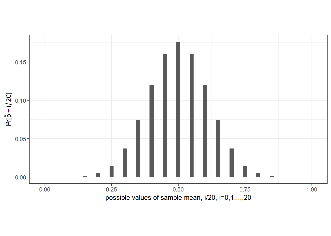

Figure 4.1: Distribution of sample mean, N=20, p=0.5.

Notice that there is non-zero probability on every possible outcome of the sample mean. This means that any reasonable decision rule that we use to reject or not reject the null hypothesis will carry a non-zero probability of rejection even when the null hypothesis is true (we call this a “Type 1 error”). For example, suppose we use the rule “Reject $p=0.5$ in favor of the alternative $p \neq 0.5$ if the frequency of heads $\hat{p}$ is less than $0.3$ or greater than $0.7$”, which seems not unreasonable. We can calculate from the table above that in using this rule, there is a probability of approximately

round(sum(Pr_phat[i/N<0.3])+sum(Pr_phat[i/N>0.7]),4)

[1] 0.0414

that we reject the null even though $p$ is in fact equal to $0.5$. We can reduce the probability of Type 1 error by allowing for a larger range for $\hat{p}$ (perhaps reject if $\hat{p} < 0.05$ or $\hat{p} > 0.95$), but then the test loses power to reject a false hypothesis (i.e., the probability of failing to reject a wrong hypothesis – a “Type 2 error” – increases). In practice, researchers usually opt for rules such that the probability of an incorrect rejection of a true hypothesis is around 0.01, or 0.05, or 0.10.

4.4 Asymptotic Analysis

Our discussion so far has been “finite sample analysis”. Asymptotic analysis refers to results that apply “in the limit”, as the sample size goes to infinity. It serves to approximate the properties of estimators in large samples. We continue to focus on the sample mean, which we now denote as $\overline{Y}_N$ to indicate the sample size used to calculate it.

4.4.1 Consistency and the Law of Large Numbers

We have mentioned the desirability of larger sample sizes. For the general problem of estimating the population mean of a random variable $Y$ with mean $\mu$ and variance $\sigma^2$ using the sample mean, we have $var[\overline{Y}_N]=\sigma^2/N \rightarrow 0$ as $N \rightarrow \infty$. Since $\overline{Y}_N$ is unbiased, and its variance collapses to zero as the sample size goes to infinity, the estimator converges to the population mean as the sample size grows larger and larger.

The convergence of $\overline{Y}_N$ to $\mu$ is not quite the same as the convergence of, say, the deterministic sequence $1/N$ to zero. In the latter case, I know that if $N$ is large enough, then $1/N$ will definitely be within a certain distance of 0. For instance, if $N>1000$, then $1/N < 0.001$ for sure. In the case of $\overline{Y}_N$, which is a sequence of random variables, we cannot make such a definite claim.

The convergence concept we use for random variables is “convergence in probability”. A sequence of random variables $X_N$ is said to converge in probability to some value $c$ as $N \rightarrow \infty$ if for any $\epsilon>0$ (no matter how small), the probability that $|X_N - c| > \epsilon$ goes to zero as $N \rightarrow \infty$. This allows for some probability that the distance between $X_N$ and $c$ exceeds $\epsilon$ at any sample size $N$, but as $N$ increases towards infinity, this probability becomes vanishingly small. We write $\mathrm{plim}X_N = c$ or $X_N \overset{p}{\rightarrow}c$. We can extend this definition to “convergence in probability to a random variable”: we say that $X_N \overset{p}{\rightarrow} Z_N$ if $X_N - Z_N \overset{p}{\rightarrow} 0$.

In the context of parameter estimation, we say that an estimator is consistent if it converges in probability to the true value of the parameter it is estimating. The sample mean $\overline{Y}_N$ is a consistent estimator for $\mu$ under quite general conditions. This result is known as a Law of Large Numbers. There are several laws of large numbers, each describing a set of conditions which, if met, guarantee the consistency of the sample mean. We state one such law below:

Theorem 4.2 (Khinchine’s Weak Law of Large Numbers, WLLN) If $\{Y_i\}_{i=1}^N$ are i.i.d. with $E[Y_i] = \mu < \infty$ for all $i$, then $\overline{Y}_N \overset{p}{\rightarrow} \mu$.

There are other kinds of convergence concepts for sequences of random variables, but for the moment we consider only convergence in probability. The theorem above is referred to as a weak law of large numbers because the convergence concept used is convergence in probability, and there are “stronger” forms of probabilistic convergence.

The following is a result concerning convergence in probability that is used frequently:

Proposition 4.1 If $g(.)$ is a continuous function, then \[ X_N \overset{p}{\rightarrow} c \Rightarrow g(X_N) \overset{p}{\rightarrow} g(c). \tag{4.9}\] That is, if $\mathrm{plim}X_N$ exists, and $g(.)$ is continuous, then $\mathrm{plim}\,g(X_N) = g(\mathrm{plim}X_N)$.

For example, if $X_N$ converges in probability to $c$, then $X_N^2 \overset{p}{\rightarrow} c^2$

Result Eq. 4.9 extends to continuous functions of multiple variables. This implies that if $X_N \overset{p}{\rightarrow} c_x$ and $Z_N \overset{p}{\rightarrow} c_z$, then

$X_N + Z_N \overset{p}{\rightarrow} c_x + c_z$,
$X_N Z_N \overset{p}{\rightarrow} c_x c_z$,
$X_N / Z_N \overset{p}{\rightarrow} c_x / c_z$, as long as $c_z$ is not zero,

and similarly for other continuous functions of $X_N$ and $Z_N$.

Example 4.2 Suppose $\{Y_i\}_{i=1}^N$ is an i.i.d. sample, with $E[Y_i]=\mu < \infty$ and $var[Y_i]=\sigma^2 < \infty$ for all $i$. We show that the biased estimator
\[ \widetilde{\sigma_{N}^{2}} = \frac{1}{N}\sum_{i=1}^N (Y_i - \overline{Y}_N)^2 = \frac{1}{N}\sum_{i=1}^N Y_i^2 - \overline{Y}_N^2 \] is consistent for the population variance $\sigma^2$. Since $\{Y_i\}_{i=1}^N$ are i.i.d., so are $\{Y_i^2\}_{i=1}^N$. Furthermore, $E[Y_i^2] = \sigma^2 + \mu^2 < \infty$, so $\frac{1}{N}\sum_{i=1}^N Y_i^2 \overset{p}{\rightarrow}\sigma^2 + \mu^2$. Since $\overline{Y}_N \overset{p}{\rightarrow} \mu$ and “power of two” is a continuous function, we have $\overline{Y}_N^2\overset{p}{\rightarrow}\mu^2$. Therefore $\widetilde{\sigma^2}$ converges in probability to $\sigma^2 + \mu^2 - \mu^2 = \sigma^2$. This example shows that consistent estimators can be biased in finite samples.

Example 4.3 Since $\widehat{\sigma_{N}^{2}} = \frac{N}{N-1}\widetilde{\sigma_{N}^{2}}$, and because $\frac{N}{N-1} \rightarrow 1$ and $\widetilde{\sigma^2} \overset{p}{\rightarrow} \sigma^2$, we have $\widehat{\sigma_{N}^{2}} \overset{p}{\rightarrow} \sigma^2$.

Example 4.4 Since both $\widehat{\sigma_{N}^{2}}$ and $\widetilde{\sigma_{N}^{2}}$ are consistent estimators for $\sigma^2$, both $(\widehat{\sigma_{N}^{2}})^{1/2}$ and $(\widetilde{\sigma_{N}^{2}})^{1/2}$ are consistent estimators for $\sigma$.

Unbiasedness, as opposed to consistency, generally does not carry over to non-linear functions of estimators. We saw earlier that $E[\hat{p}^{2}] > p^{2}$ despite $E[\hat{p}] = p$. The following is another example.

Example 4.5 Unbiasedness of an estimator $\hat{\theta}$ for some parameter $\theta$ does not imply unbiasedness of $\hat{\theta}^{1/2}$ for $\theta^{1/2}$. In fact, we can see from $var[\hat{\theta}^{1/2}] = E[\hat{\theta}] - E[\hat{\theta}^{1/2}]^2$ that $E[\hat{\theta}^{1/2}]^2 < E[\hat{\theta}]$. If $\hat{\theta}$ is unbiased, we have $E[\hat{\theta}^{1/2}]^2 < \theta$. Taking square roots then gives \[ E[\hat{\theta}^{1/2}] < \theta^{1/2}. \] Both $(\widehat{\sigma_{N}^{2}})^{1/2}$ and $(\widetilde{\sigma_{N}^{2}})^{1/2}$ are biased (but consistent) estimators for $\sigma$.

It may seem that unbiasedness (together with efficiency) is a more relevant way to judge an estimator than consistency since we never have infinite sample sizes, but consistency is still useful as it captures the idea of convergence to the population parameter as sample size increases. Furthermore, in more complex applications it can be difficult or impossible to find unbiased estimators, but straightforward to find consistent ones. We have also seen that it is easy to find consistent estimators of continuous functions of parameters once we have consistent estimators for the parameters.

Earlier we derived the distribution of the sample mean in the coin toss example, and calculated this distribution for a fair coin with sample size 20. We repeat this exercise, this time for a coin with $p=0.25$, for sample sizes of 5, 10, 20, 100, 200 and 400. We present the probability distribution functions graphically in Fig. 4.2. The convergence in probability of the sample mean to the true value of $p$ can be seen in these graphs.

p <- 0.25   # Assume probability of heads = 0.25
samplesize <- c(5,10,20,100,200,400)
pdfs <- list()  # to store our plots in the loop
for (j in 1:6){
  N <- samplesize[j]
  i <- 0:N
  phat <- 0:N/N    
  Pr_phat <- choose(N,i)*p^i*(1-p)^(N-i)
  data <- data.frame(phat=phat,Pr_phat=Pr_phat)
  pdfs[[j]] <- ggplot(data,aes(x=phat,y=Pr_phat))+
          geom_bar(stat="identity", width=0.005)+
          ylab("")+xlab(paste0('N=',N)) + theme_minimal() + 
          theme(axis.text=element_text(size=7),
                axis.title=element_text(size=7))
}
(pdfs[[1]] | pdfs[[2]] | pdfs[[3]]) / 
(pdfs[[4]] | pdfs[[5]] | pdfs[[6]])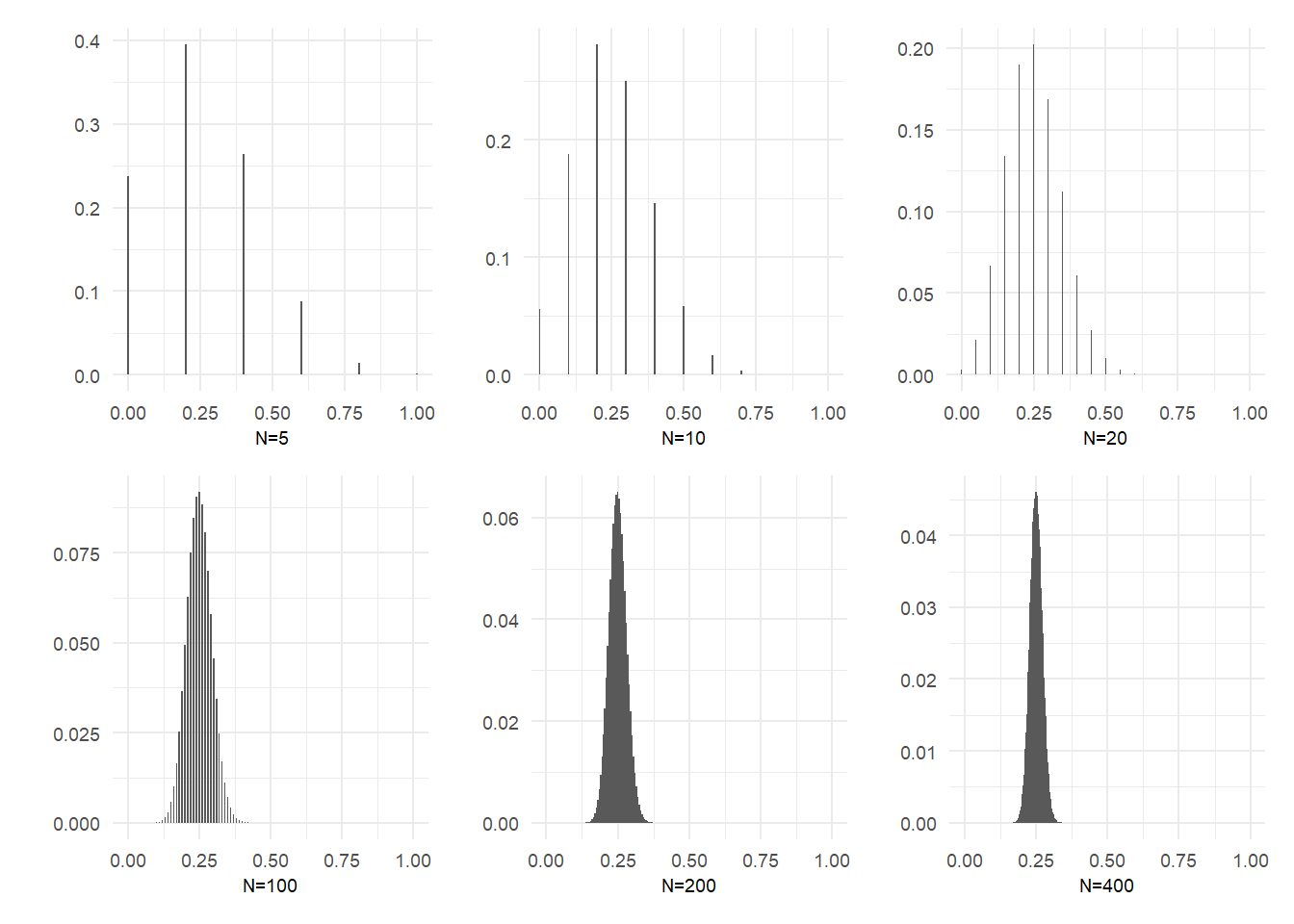

Figure 4.2: Consistency of sample mean to p=0.25.

4.4.2 Asymptotic Normality

The distribution of the sample mean in the example above, with $p=0.25$, is unsurprisingly skewed in small samples because of the low probability of heads relative to tails. However, the shape of the distribution appears to quickly becomes quite symmetric as sample size grows, and appears to converge to a familiar bell-shaped distribution. Of course, in the limit the distribution collapses to a degenerate one with all of the probability at $p=0.25$. This is because the variance of the sample mean, $var[\hat{p}]=p(1-p)/N$ goes to zero as $N \rightarrow \infty$. Suppose, however, that we scale the sample mean (after subtracting $p$) by $\sqrt{N}$, i.e., suppose we look at the distribution of \[ \sqrt{N}(\hat{p}-p). \tag{4.10}\] This random variable has mean 0 and a non-collapsing variance $Np(1-p)/N=p(1-p)$. We can then talk about the shape of Eq. 4.10 as $N \rightarrow \infty$ without the distribution collapsing to a single point. The plots below show the same distributions as above, but after centering and scaling as in Eq. 4.10.

p <- 0.25   # Assume probability of heads = 0.25
samplesize <- c(5,10,20,100,200,400)
pdfs <- list()  # to store our plots in the loop
for (j in 1:6){
  N <- samplesize[j]
  i <- 0:N
  phat <- 0:N/N    
  phat_scaled <- sqrt(N)*(phat - p)
  Pr_phat_scaled <- choose(N,i)*p^i*(1-p)^(N-i)
  data <- data.frame(phat_scaled=phat_scaled,Pr_phat_scaled=Pr_phat_scaled)
  pdfs[[j]] <- ggplot(data,aes(x=phat_scaled,y=Pr_phat_scaled)) + 
          geom_bar(stat="identity", width=0.05) + ylab("") + 
          xlab(paste0('N=',N)) + xlim(c(-2.5,2.5)) + theme_minimal() + 
          theme(axis.text=element_text(size=8),
                axis.title=element_text(size=7))
}
(pdfs[[1]] | pdfs[[2]] | pdfs[[3]]) / 
(pdfs[[4]] | pdfs[[5]] | pdfs[[6]])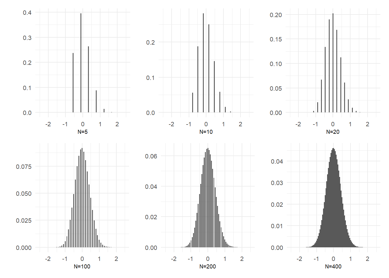

Figure 4.3: Convergence of distribution to normal (pdf view).

The distributions appear to take the shape of a normal distribution as sample size increases. Of course, the sample mean in the coin toss example is a discrete random variable, whereas a normally distributed random variable is a continuous one. The notion of a discrete pdf converging to a continuous one is best thought of in terms of their cdfs. In the figure below, we juxtapose the cdf of the distribution of $\sqrt{N}(\hat{p}-p)$ at $N=400$ (which is a step function) with the cdf of the normal distribution with mean 0 and variance $p(1-p)$ where $p=0.25$.

p <- 0.25   # Assume probability of heads = 0.25
N = 400
i <- 0:N
phat <- 0:N/N
phat_scaled <- sqrt(N)*(phat - p)
cdf_phat_scaled <- cumsum(choose(N,i)*p^i*(1-p)^(N-i))
cdf_norm <- pnorm(phat_scaled,0,sqrt(p*(1-p)))
data1 <- data.frame(phat_scaled=phat_scaled,
                   cdf_phat_scaled=cdf_phat_scaled)
data2 <- data.frame(phat_scaled=phat_scaled,
                    cdf_norm=cdf_norm)
ggplot()+
  geom_step(data=data1,aes(x=phat_scaled,y=cdf_phat_scaled,color="blue"),
           direction="vh")+
  geom_line(data=data2,aes(x=phat_scaled,y=cdf_norm,color="red"))+
  xlab(TeX("$\\sqrt{N}(\\hat{p}-p), N = 400, p=0.25"))+ylab("")+
  xlim(c(-2.5,2.5))+ylim(c(0,1.1)) + theme_minimal() + 
  theme(axis.text=element_text(size=7), axis.title=element_text(size=8)) +
  scale_colour_manual(
       name = '', 
       values = c('blue'='blue','red'='red'), 
       labels = c('emp. cdf. phat_scaled','cdf. N(0,p(1-p))'))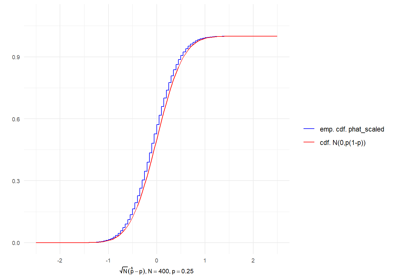

Figure 4.4: Convergence of distribution of sample mean to normal (cdf view).

4.4.3 The Central Limit Theorem

The convergence of the cdf of the (centered and scaled) sample mean in the coin toss example to a normal cdf is an instance of the Central Limit Theorem (CLT), a key result in probability theory. As with the Law of Large Numbers, there are many CLTs, each listing out a set of conditions under which convergence to normality is guaranteed. We state one such CLT:

Theorem 4.3 (Lindeberg-Levy CLT) If $\{Y_i\}_{i=1}^N$ are i.i.d. with $E[Y_i] = \mu < \infty$ and $var[Y_i] = \sigma^2 < \infty$ for all $i$, then \[ \sqrt{N}(\overline{Y}_N - \mu) \;\overset{d}{\rightarrow} \;\mathrm{Normal}(0,\sigma^2) \] where $\overset{d}{\rightarrow}$ means convergence in distribution, meaning that the cdf of the random variable on the left converges point-wise to the cdf of the distribution indicated on the right.

Our plots of the distribution of $\sqrt{N}(\hat{p}_N - p)$ in the coin toss example suggests convergence in distribution to $\mathrm{Normal}(0,p(1-p))$. The sample $\{Y_i\}$ in the coin toss example does in fact meet the requirements of the Lindeberg-Levy CLT, so we can claim that $\sqrt{N}(\hat{p}_N - p) \overset{d}{\rightarrow} \mathrm{Normal}(0,p(1-p))$

Sometimes we want to indicate that a sequence of random variables $X_N$ converges in distribution to the cdf of some random variable $X$. To so do, we write $X_N \overset{d}{\rightarrow} X$.

Proposition 4.2 (Properties of convergence in distribution)

If $g(.)$ is a continuous function and $X_N \overset{d}{\rightarrow} X$, then $g(X_N) \overset{d}{\rightarrow} g(X)$.
If $X_N \overset{p}{\rightarrow} X$, then $X_N \overset{d}{\rightarrow} X$.
If $a_N \overset{p}{\rightarrow} a$ and $X_N \overset{d}{\rightarrow} X$, then $a_N X_N \overset{d}{\rightarrow} aX$.

Example 4.6 If $X_N \overset{d}{\rightarrow} X \sim N(0,1)$, then $X_N^2 \overset{d}{\rightarrow} X^2 \sim \chi_{(1)}^2$, since the square of a standard normal is $\chi^2(1)$.

Example 4.7 If $\sqrt{N}(\overline{Y}_N - \mu) \overset{d}{\rightarrow} \mathrm{Normal}(0,\sigma^2)$ and $s_N^2$ is any consistent estimator of $\sigma^2$, then $1/s_N = (1/s_N^2)^{1/2}$ converges in probability to $1/\sigma$, and therefore \[ t = \frac{\sqrt{N}(\overline{Y}_N - \mu)}{s_N} = \frac{\overline{Y}_N - \mu}{\sqrt{s_N^2/N}}\overset{d}{\rightarrow} N(0,1). \tag{4.11}\]

If $\sqrt{N}(\overline{Y}_N - \mu) \overset{d}{\rightarrow} \mathrm{Normal}(0,\sigma^2)$, we would be justified, in large enough samples, to say that the distribution of $\sqrt{N}(\overline{Y}_N - \mu)$ is approximately $\mathrm{Normal}(0,\sigma^2)$, or that $\overline{Y}$ is approximately $N(\mu,\sigma^2/N)$. This last statement is sometimes written $\overline{Y}_N\overset{a}{\sim}N(\mu,\sigma^2/N)$, where the “$a$” stands for “approximately” (some take “$a$” to stand for “asymptotically”).

Result Eq. 4.11 is useful for hypotheses testing when one is unable or unwilling to make an assumption regarding the distribution of the sample. Suppose $\{Y_i\}_{i=1}^N$ is an i.i.d. sample with $E[Y_i]=\mu$ and $var[Y_i]=\sigma^2$. The sample mean $\overline{Y}$ is a consistent estimator for $\mu$ and $\widehat{\sigma^2}=\frac{1}{N-1}\sum_{i=1}^N (Y_i-\overline{Y})^2$ is a consistent estimator for $\sigma^2$. To test the null hypothesis $H_0:\mu=\mu_0$, where $\mu_0$ is some numerical value, we need to compute the distribution of the sample mean, but you cannot do this unless you know the distribution of each $Y_i$. Result Eq. 4.11, however, tells us that if our sample size is large enough, then under the null hypothesis, \[ t = \frac{\overline{Y}_N - \mu_0}{\sqrt{s_N^2/N}} \overset{a}{\sim} \mathrm{Normal}(0,1). \tag{4.12}\] It suggests that we use the decision rule “reject the null if $|t|>c_\alpha$” where $c_\alpha$ is that value such that $\mathrm{Pr}[|t|>c_\alpha]=\alpha$, where $\alpha$ is the chosen “level of significance” of the test, i.e., the probability of rejecting the null when it is true, and where the value $c_\alpha$ is found from the normal distribution. For 0.01, 0.05, 0.10 levels of significance, the appropriate values of $c_\alpha$ are approximately

round(qnorm(c(0.995, 0.975, 0.95)),3)

[1] 2.576 1.960 1.645

respectively. The 0.05 level of significance test, in particular, says to reject $H_0:\mu=\mu_0$ if the absolute distance from the sample mean to the hypothesized value $\mu_0$ is more than $1.96$ (or approximately $2$) standard errors.

A test based on the statistic in Eq. 4.12 and rejection values (or ‘critical values’) based on the $\mathrm{Normal}(0,1)$ distribution, would be an approximate test in the sense that the true significance level may not be exactly $\alpha$, as intended. Nonetheless, it is a way forward in a situation where an exact test is unavailable. Even where the exact distribution is available, such as in our coin toss example, the approximate test using Eq. 4.12 can be a convenient approximation.

Example 4.8 Earlier we showed an example of $20$ tosses of three coins, where the true value of $p$ for coins $1$, $2$, and $3$ are $0.5$, $0.6$, and $0.9$ respectively. We replicate the results below, this time also computing the corresponding t-statistics for the hypothesis $H_0:p=0.5$, i.e., we compute \[ t = \frac{\hat{p}-0.5}{\sqrt{\frac{\hat{p}(1-\hat{p})}{N-1}}} \]

set.seed(13)   # Initialize random number generator for replicability
N <- 20
Coin1 <- rbinom(N,1,0.5)   # 20 tosses of a fair coin
Coin2 <- rbinom(N,1,0.6)   # 20 tosses of a slightly unfair coin
Coin3 <- rbinom(N,1,0.9)   # 20 tosses of a very warped coin!
Tosses <- rbind(Coin1, Coin2, Coin3)  # place outcomes into three rows
p_hat <- apply(Tosses,1,mean) # apply mean function to each row of Tosses
var_p_hat <- p_hat*(1-p_hat)/(N-1) # as per formula derived in notes
se_p_hat <- sqrt(var_p_hat)
t_stat <- (p_hat-0.5)/se_p_hat
p_val <- 2*(1-pnorm(t_stat,0,1))
# Output
d <- cbind(p_hat,se_p_hat,t_stat,p_val)
round(d,4)

      p_hat se_p_hat t_stat  p_val
Coin1  0.65   0.1094 1.3708 0.1704
Coin2  0.70   0.1051 1.9024 0.0571
Coin3  0.85   0.0819 4.2726 0.0000

Using the asymptotic tests, we make the following (approximate) conclusions:

we (correctly) fail to reject the hypothesis that Coin 1 is fair at any of the usual levels of significance.
we (correctly) reject the hypothesis for Coin 2 at $0.1$ level of significance, but (incorrectly) fail to reject at the $0.05$ level of significance.
Fairness of Coin 3 is resoundingly (and correctly) rejected at all conventional levels of significance.

The result for Coin 2 illustrates the fact that it can be hard to reject a mildly incorrect hypothesis. All tests have poor power in such cases. The results for Coin 1 and Coin 3 turned out to be correct in this example, but it should be remembered that there were non-zero probabilities of rejecting fairness for Coin 1, and not rejecting fairness for Coin 3.

In addition to the t-statistic, we also compute the p-value, i.e., the probability that the t-statistic, prior to realization, would exceed the value realized, in absolute terms. We reject a hypothesis at $\alpha$ level of significance if the p-value is smaller than $\alpha$.

The statistic in Eq. 4.12 is sometimes called a $z$-statistic, and often called a t-statistic because its exact distribution would be the t-distribution (with degree of freedom $N-1$) if the sample were normally distributed, i.e., if $Y_i \sim \mathrm{Normal}(\mu,\sigma^2)$ for all $i$, then \[ t = \frac{\overline{Y}_{N}-\mu}{\sqrt{\widehat{\sigma_{N}^{2}}/N}}\;\;\sim\;\;t_{(N-1)}\,. \] Since $Y_{i}$ is not normal in the coin toss example, this result does not apply, and we rely on the asymptotic result. Of course, the t-distribution is itself approximately standard normal when $N$ is large, so in this case, the $t$-statistic converges to the standard normal for two reasons: because of the central limit theorem, and because the t-distribution anyway converges to the standard normal as the degree of freedom goes to infinity. The usefulness of result Eq. 4.12 is in its applicability regardless of the distribution of the sample, when sample sizes are large enough.

4.5 Exercises

Exercise 4.1 Prove the last equality in Eq. 4.6.

Exercise 4.2 Prove the last equality in Eq. 4.4.

Exercise 4.3 Suppose $\hat{\theta}$ is an unbiased estimator. Prove that $g(\hat{\theta})$ is an unbiased estimator of $g(\theta)$ if $g(\theta)$ has the form $g(\theta)=a+b\theta$.

Exercise 4.4 A function $g(.)$ that is differentiable and concave has the property that the function lies on or under every tangent line. The functions $g(x)=\sqrt{x}$, $x \geq 0$ and $g(x)=\mathrm{ln}x$, $x>0$ are both examples of concave functions. Follow the steps below to prove Jensen’s Inequality, which says that if $g(.)$ is concave, then \[ E[g(X)] \leq g(E[X]). \] Step 1: Let $l(x)=a+bx$ be the tangent line of the concave function $g(x)$ at the point $(E[X],g(E[X]))$, i.e., $l(x)=a+bx$ satisfies \[ l(x)=a+bx \geq g(x) \;\; \text{ and } \;\; l(E[X])=a+bE[X] = g(E[X])\,. \] Step 2: Prove Jensen’s Inequality by using the fact that if $f_1(x) \leq f_2(x)$, then $E[f_1(X)] \leq E[f_2(X)]$.

Exercise 4.5 Prove the last equality in Eq. 4.7.

Exercise 4.6 For the coin toss example, compute the probability of rejecting the null hypothesis $H_0: p=0.5$ using the rule “Reject $H_0$ if $\hat{p}=\overline{Y}$ is strictly greater than 0.7 or strictly less than 0.3” for values of $p = 0.05, 0.1, ..., 0.90, 0.95$ when $N=20$. Plot these probabilities against $p$. Repeat the exercise for $N=50$.

The Bias-Variance Trade-off

Exercise 4.7 It can be shown that if $Y_i$, $i=1,2,...,N$ are i.i.d. draws from a normal distribution with mean $\mu$ and variance $\sigma^2$, then the variance of the unbiased variance estimator $\widehat{\sigma^2}$ defined in Eq. 4.5 is $var[\widehat{\sigma^2}]=\frac{2\sigma^4}{N-1}$. Because $\widehat{\sigma^2}$ is an unbiased estimator, its MSE is also $\frac{2\sigma^4}{N-1}$.

Show that the biased estimator $\widetilde{\sigma^2}$ defined in Eq. 4.4 has a smaller variance than $\widehat{\sigma^2}$.
Show that $\mathrm{MSE}[\widetilde{\sigma^2}] = \frac{2N-1}{N^2}\sigma^4$.
Show that $\mathrm{MSE}[\widetilde{\sigma^2}] < \mathrm{MSE}[\widehat{\sigma^2}]$.

This is an example where MSE can be improved by trading off some bias for a reduced variance. Note that the arguments here have assumed that $Y$ is normally distributed.

Exercise 4.8 Consider the coin toss example with $N=10$. Let $\hat{p} = (1/10)\sum_{i=1}^{10} Y_{i}$, and let $\widetilde{p}=(1/11)\sum_{i=1}^{10} Y_{i}$ be an alternative estimator. We know $\hat{p}$ is unbiased, and therefore $\widetilde{p}$ is biased (downwards).

Show that the variance of $\widetilde{p}$ is $(10/121)p(1-p)$ (which is lower than $var[\hat{p}] = p(1-p)/10$).
Find the $MSE$ of $\hat{p}$.
Find the $MSE$ of $\widetilde{p}$.
Show that $MSE[\widetilde{p}] < MSE[\hat{p}]$ if $p < 21/31$.

Remark: The estimator $\widetilde{p}$ is biased but it has a lower variance than the unbiased $\hat{p}$. It turns out that this bias-variance trade-off is favorable toward minimizing MSE only if $p < 21/31$. If it is believed that $p<21/31$, and the objective is minimizing MSE, then the alternate estimator may be preferred.

4.6 Prediction

Suppose you have an iid sample $Y_{1}$, $Y_{2}$, … $Y_{N}$ of draws from random variable $Y$ with mean $E[Y]=\mu$ and variance $var[Y]=\sigma^{2}$. Your interest is in predicting the value of the next independent draw $Y_{N+1}$. In the previous chapter we learnt that the point prediction that minimizes the mean squared prediction error is the expectation conditional on the information set $X$. In this application, the $X$ is just your sample $Y_{1}$, $Y_{2}$, …, $Y_{N}$ and the optimal prediction is the conditional expectation $E[Y_{N+1}|Y_{1}, ..., Y_{N}]$. Since it is assumed that the sample is iid, the conditional mean reduces to the unconditional mean $E[Y_{N+1}] = \mu$. You decide to estimate the sample mean from your iid sample, and use this as your predictor, i.e., you choose \[ \widehat{Y}_{N+1} = \overline{Y} = \frac{1}{N}\sum_{i=1}^{N} Y_{i}\,. \] What is the MSPE for this predictor? The conditional MSPE when predicting $Y_{N+1}$ using $\overline{Y}$ estimated over $Y_{1}$, …, $Y_{N}$ is \[ \begin{aligned} MSPE(Y_{N+1}, \overline{Y}|X) &= E[(Y_{N+1}-\overline{Y})^{2}|X] \\ &= E[(Y_{N+1}-\mu + \mu - \overline{Y})^{2}|X]\\ &= E[(Y_{N+1}-\mu)^{2}| X] + E[(\mu - \overline{Y})^{2}|X] + 2E[(Y_{N+1} - \mu)(\mu - \overline{Y})|X] \\ &= E[(Y_{N+1}-\mu)^{2}] + (\mu - \overline{Y})^{2} + 2(\mu - \overline{Y})E[(Y_{N+1} - \mu)|X] \\ &= var[Y_{N+1}] + (\overline{Y} - \mu)^{2} \end{aligned} \] where we have used the assumption that $Y_{N+1}$ is independent of the sample $X = \{Y_{1}, \dots, Y_{N}\}$. Taking expectation over $X$, we get the unconditional MSPE to be \[ \begin{aligned} MSPE(Y_{N+1}, \overline{Y}) &= E[MSPE(Y_{N+1}, \overline{Y}|X)] \\ &= E[var[Y_{N+1}]] + E[(\overline{Y} - \mu)^{2}] \\ &= var[Y_{N+1}] + var[\overline{Y}]\,. \end{aligned} \] That is, the MSPE is \[ MSPE(Y_{N+1}, \overline{Y}) = \sigma^{2} + \frac{\sigma^{2}}{N}\,. \] The first term is due to the fact that we are predicting a new observation outside of the sample. The second term comes from the variance of the sample mean. We can estimate the MSPE by replacing $\sigma^{2}$ with $\widehat{\sigma^{2}}$, i.e., \[ \widehat{MSPE}(Y_{N+1}, \overline{Y}) = \widehat{\sigma^{2}} + \frac{\widehat{\sigma^{2}}}{N}\,. \tag{4.13}\] Often the prediction is reported as \[ \text{prediction} \pm 2 \sqrt{\widehat{MSPE}}. \] This is often called the “0.95 Prediction Interval”.³ Some people use 1.96 instead of 2.

Two remarks: first, since the $MSPE(Y_{N+1}, \overline{Y}|X) = E[(Y_{N+1}-\hat{\mu})^{2}]$, one might be tempted to estimate it with \[ \frac{1}{N}\sum_{i=1}^{N} (Y_{i} - \overline{Y})^2\, \;\; \text{ or } \;\; \frac{1}{N-1}\sum_{i=1}^{N} (Y_{i} - \overline{Y})^2 \] This is, of course, merely an estimate of $\sigma^{2}$, and would underestimate the MSPE. This is because you are using “in-sample” or “training” data to estimate MSPE, and the result does not generalize to out-of-sample predictions.

4.6.1 Exercises

The following questions are based on the above prediction example.

Exercise 4.9 Explain why using \[ \widehat{\sigma^{2}} = \frac{1}{N-1}\sum_{i=1}^{N}(Y_{i}-\overline{Y})^{2} \] in Eq. 4.13 results in an unbiased estimate of $\widehat{MSPE}(Y_{N+1}, \overline{Y})$.

Exercise 4.10 Suppose instead of the estimating the MSPE using Eq. 4.13, you did the following instead: divide your sample of $N$ observations into two subsamples of sizes $N_{1}$ and $N_{2}$. In particular, divide your $N$ observations into observations $i = 1, 2, ..., N_1$ and $j = N_1 + 1, N_1 + 2, ..., N_1+N_2$. (Perhaps $N_{2}$ might be $N/5$, but the size of split is not so important). Then estimate $\mu$ over the $N_{1}$ sample, and estimate your MSPE over the $N_{2}$ sample, i.e., \[ \widetilde{\mu} = \frac{1}{N_{1}}\sum_{i=1}^{N_{1}} Y_{i} \;\; \text{ and } \;\; \widetilde{MSPE}(Y_{N+1},\widetilde{\mu}) = \frac{1}{N_{2}}\sum_{j=N_1+1}^{N_{1}+N_{2}} (Y_{j}-\widetilde{\mu})^{2}\,. \] Show that $\widetilde{MSPE}(Y_{N+1},\widetilde{\mu})$ is an unbiased estimator of $MSPE(Y_{N+1}, \widetilde{\mu})$, which is \[ MSPE(Y_{N+1}, \widetilde{\mu}) = \sigma^{2} + \frac{\sigma^{2}}{N_{1}}\,. \] Remark: An “advantage” of this method of estimating $MSPE$ is that we did not have to estimate $\sigma^{2}$, but this is a hardly an advantage since we have unbiased estimators of $\sigma^{2}$. The major disadvantage of this method is that you are estimating the sample mean using a smaller sample, which increases its sampling variability, and increases the MSPE. Since we have easily derived the formula for the MSPE in this simple application, there is no advantage to the method proposed here. However, in more advanced applications, the form of the MSPE might not be so easy to derive. In those applications, and assuming a large enough sample size, it may be advantageous to estimate the MSPE in the manner described in this exercise. The “cross-validation” method used in machine learning is an extension of the method described here. The method proposed here may also be useful in the situation where the loss function is not squared error.

Exercise 4.11 Suppose instead of the sample mean, you use some other (possibly biased) estimator $\hat{g}(X)$ where $X = \{Y_{1}, \dots, Y_{N}\}$ to predict an independent observation $Y_{N+1}$. Show that the $MSPE$ is \[ MSPE(Y_{N+1}, \hat{g}(X)) = \sigma^{2} + var[\hat{g}(X)] + (E[\hat{g}(X)] - \mu)^{2}\,. \] Hint: Write \[ \begin{aligned} MSPE(Y_{N+1}, \hat{g}(X)) &= E[(Y_{N+1} - \hat{g}(X))^{2}] \\ &= E[(Y_{N+1} - \mu + \mu - E[\hat{g}(X)] + E[\hat{g}(X)] - \hat{g}(X))^{2}] \\ &= E[A^{2} + B^{2} + C^{2} + 2AB + 2AC + 2BC] \end{aligned} \] where $A = Y_{N+1} - \mu$, $B = \mu - E[\hat{g}(X)]$ and $C=E[\hat{g}(X)] - \hat{g}(X))$. Then compute the expectation by first taking expectations conditional on $X$, then take expectations over $X$. When taking expectations conditional of $X$, $\hat{g}(X)$ is fixed. You should find that the last three terms drop out, and the $E[A^{2}] = \sigma^{2}$, $E[B^{2}]$ is the squared bias, and $E[C^2]$ is the variance of $\hat{g}(X)$. When $\hat{g}(X)$ is the sample mean, which is unbiased, the MSPE reduces to $\sigma^{2} + \sigma^{2}/N$.

Exercise 4.12 In the coin toss example, suppose you want to use $N$ independent coin tosses to predict the outcome of the next coin toss. Suppose your loss function is squared error. What is your optimal point prediction?

Exercise 4.13 Continuing with the coin toss example, suppose you have estimated the probability of Heads to be $\hat{p}$. Suppose now that your prediction $\widehat{Y}_{N+1}$ for the next toss must be either ‘heads’ or ‘tails’ (i.e., 1 or 0, you cannot give fractional answers) and your loss function is “0-1”, meaning that your loss is $1$ if you are wrong, and $0$ if you are right, i.e., \[ L(Y_{N+1}, \widehat{Y}_{N+1}) = \begin{cases} 1, &\text{if $Y_{N+1} \neq \widehat{Y}_{N+1}$} \\ 0, &\text{if $Y_{N+1} = \widehat{Y}_{N+1}$}\,. \end{cases} \] Show that your optimal prediction is $\widehat{Y}_{N+1} = 1$ if $\hat{p} \geq 0.5$, $\hat{Y}_{N+1} = 0$ otherwise.

Hint: You want to choose $\widehat{Y}_{N+1} = 1 \text{ or } 0$ to minimize your expected loss, which is \[ L(Y_{N+1} = 1, \widehat{Y}_{N+1}) Pr[Y_{N+1} = 1] + L(Y_{N+1} = 0, \widehat{Y}_{N+1}) \Pr[Y_{N+1} = 0]\,. \] Compare this value for the cases $\widehat{Y}_{N+1} = 1$ and $\widehat{Y}_{N+1} = 0$ and ask: which choice minimizes expected loss when $\Pr[Y_{N+1} = 1] \geq 0.5$? Which choice minimizes expected loss when $\Pr[Y_{N+1} = 0] < 0.5$?

The square root of the estimator variance is the standard error of the estimator, and can be thought of as a measure of the size of the estimation error one might expect to make.↩︎
An example of a non-linear estimator is the geometric mean $(Y_1 \times Y_2 \times \cdots \times Y_N)^{1/N}$ which, incidentally, is biased downwards, and can only be used for positive random variables.↩︎
The 0.95 Confidence Interval, on the other hand, uses only the sample error from estimating the mean, i.e., \[ \hat{\mu} \pm 2 \sqrt{\widehat{\sigma^2}/N}\,. \] This is the 0.95 confidence interval for the sample mean, and is a measure of uncertainty about the estimate of the sample mean, not the prediction.↩︎