1  A Brief Introduction to R

1.1 Getting Set Up

First download and install the R software from The R Project for Statistical Computing website. Then download and install RStudio from the RStudio website (go to Products, RStudio under the Open Source tab, and download the Open Source Edition of RStudio Desktop). RStudio is an “integrated development environment” (IDE) comprising a set of programs that help you to develop and run R code. You do not need RStudio to run R, but this is what we will do.

When you first run RStudio, you will see an RStudio desktop open up with three or four windows. There will be one with tabs such as Files, Plots, Packages, Help, and Viewer, another window with tabs marked Console, Terminal, Jobs, and a third window with Environments, History, Connections, and other tabs. If you go to the menu and select File>New File>R Script, a fourth window will open up with an Untitled1 tab. This is the Editor window, and the Untitled1 tab is a blank R Script file.

You will issue commands in the Console tab, or write your instructions in a R script file and execute them from the Editor window. If you ask R to display the results o calculations, these will show up in the Console tab. Graphics produced will show up in the Plots tab. Objects created will be listed in the Environment tab. Executing commands from an R script is best practice; you can save the commands, modify them, correct errors and redo computations easily. Use the console to test commands, make inquiries of objects, and for other one-off actions.

Activity: Go to your console tab, type x <- 4.5 and press enter. Type x and enter.

x <- 4.5
x

[1] 4.5

You have just used the assignment operator <- to create an object named x containing the number 4.5.¹ The object x now appears in your Environment tab. You can also use the = operator, but we almost always use <- for assignment and = when giving values to parameters in functions. The second line prints the value of x to your console.

If you make a calculation, say 2+2, and don’t assign the result to a name, the result of that calculation is displayed in the console window, but is thereafter inaccessible, lost in computer memory until overwritten by R.

Activity: Open a new R Script in the Editor window (or use the ‘untitled’ script if it is already open), and type in the following lines.

# Any line or part of line following a '#' is ignored by R
# We use this feature to add comments to code

y <- seq(1,10)         # Create an integer sequence from 1 to 10
plot(y,1/y,type='l')   # Create a line plot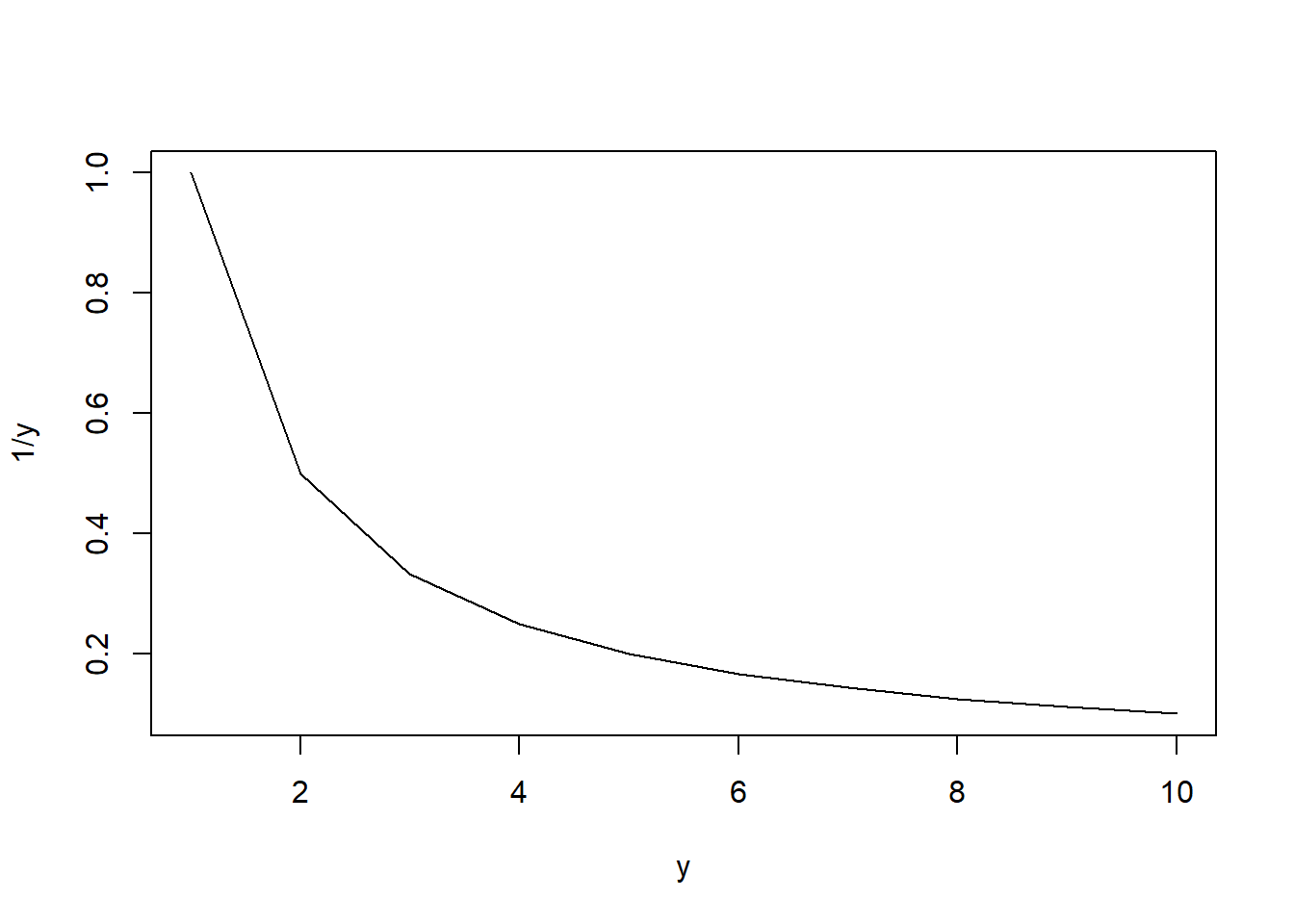

On your Editor window, click on the Source button (alternatively, select all lines and hit Ctrl+Enter). This will cause all of the lines in the R script to run one after the other. A line plot will appear on your Plots tab. If you select Export>Copy to Clipboard, the plot appears in a pop-up window. If you click Copy Plot, the plot is placed on your clipboard and you can then paste the plot into, say, a Word document. New plots are placed over current plots. Use the arrows in the plot window to go back and forth between plots. Press the red circle with a white X to erase the current plot. Press the broom icon to erase all plots. To save your script, click on the floppy disk icon and save the file with an appropriate name. The saved file will have the “.R” extension.

In R, you store your data in vectors, matrices, lists, data frames (and variants of it), and time series objects (and variants of it). These are different data structures, i.e., different ways that R can organize your data.

You will work with different kinds of data types, including integer (whole numbers, without decimals), double (or floating-point for numbers with decimals), character (for text data), logical (or boolean, to indicate TRUE or FALSE), and complex (for complex numbers). Numbers such as 1 and 2 can be stored either as integers or doubles. To force a whole number to be an integer, we append an L after the number, e.g., 1L. Integer and double are also collectively known as numeric data types. There is also a factor data type for categorical data.

All actions in R are carried out using functions such as seq() and plot(), and operators such as <- and : (operators are actually also functions). Functions in R are sets of instructions designed to perform certain tasks. Pre-written R functions are organized into packages. Every installation of R comes with some packages pre-installed (including the base, datasets, graphics and stats packages) and which are automatically loaded every time you start R. There are many other packages written by independent programmers that provide additional functionality and that are not pre-installed in R. To access these functions, you have first to install the package into your R installation. You can then load the package into any R session that requires the functions in that package. Finally, you can write your own functions.²

To find out more about any given R function, enter ? function_name into the console and the relevant documentation will come up, e.g.,

? seq  # Enter this and see what happens
? `:`  # With this sort of operators, you have to use surround them by backticks

As we mentioned earlier, objects that you create go into your “environment”. To see what is in your environment, use ls(). To remove all objects in your environment, use rm(list=ls()). Try the following line-by-line.

ls()            # ls ~ list objects
rm(list=ls())   # rm ~ remove. Environment is now clear.

Most of the data that you work with will be imported from an external files (.csv, .xlsx, etc.) and stored data frames. We will import some later. You will also want to “create” data within R. For instance, you may want to create a sequence of integers, or a value that will be used as a constant in your work, or generate a sequence of random numbers and so on.

1.2 Data Types

Activity: Run the following commands and queries as suggested, line by line.

## The following illustrate some of the major data types in R
a1 <- 1L            # Integer  
a2 <- 4             # Integer or Double?
a3 <- 2.3           # Double 
a4 <- TRUE          # Logical
a5 <- "Two"         # Character, making up a "string"
a6 <- "12"          # Another string
a7 <- 2+1i          # Complex

## Use typeof() to query the data type of the object
typeof(a1)         # Try with the others objects you created

## The is.integer(), is.double(), is.numeric(), is.character(), is.complex()
## functions make more specific queries as to the object's data type. An example 
## is shown. Try each of the query function on each of the objects above.
is.integer(a2)    
## In some cases, you can "coerce" R to change data types using functions like 
## as.integer(), as.double(), as.numeric(), as.logical(), as.character(), as.complex(). 
## An example is shown below. Try these functions of each of the objects created so far.
as.integer(a4)      

## Sometimes R will do the coercion for you
3 + TRUE

There are special values in R:

• NA stands for “Not Available” or “Missing”. It is by default a logical datatype, but can be converted to other data types.
• NULL is an empty object, with no datatype.
• Inf stands for “Infinity” and comes about when you do operations like 1/0. It is by default a numeric datatype (specifically double, but coerce-able to complex).
• NaN stands for “Not a Number” and comes about when you do operations like Inf-Inf. It is, ironically, of numeric datatype by default (specifically double, coerce-able to complex).

The following are examples of how these values can arise, or how they may be used.

1/0       # This will give you Inf
Inf - Inf # Gives NaN. Inf - Inf is NOT equal to zero
0/0       # Also gives NaN. 0/0 is NOT equal to one. Please.
a <- NA   # Basically saying the data that's suppose to be there is missing

NULL, NA, Inf and NaN are reserved words. You cannot use them as names of objects. Other reserved words include: if, else, while, repeat, for, next, in, function, break, TRUE, FALSE.

Computers can only store real numbers up to some degree of accuracy:

Activity: The sqrt() function returns the square root of a number. Execute the following code. Do the results surprise you?

sqrt(2)
sqrt(2)*sqrt(2)
sqrt(2)*sqrt(2) == 2  # use == to make equality comparisons
sqrt(2)*sqrt(2) - 2 

The e-16 in the output stands for \(\times 10^{-16}\). Computers, of course, cannot store irrational numbers to infinite accuracy, and this can lead to surprising results when making comparisons, or inaccurate results when performing complicated tasks that involve a very large number of calculations. For now, just bear this in mind. The degree of accuracy is generally not going to be an issue for us (except when making comparisons).

1.2.1 Arithmetic and Logical Operators

The arithmetic operators include: Addition (+), Subtraction (-), Multiplication (*), Division (/), and Exponent (^). The usual operator precedence apply: operations in parentheses are evaluated first, followed by ^, followed by (*,/), followed by (+/-). Ties between multiplication and division, and between addition and subtraction, are broken by evaluating from left to right. Always use parentheses when in doubt.

Activity: Enter \(8 / 2 * (2+2)\). Do you agree with the result?

 8 / 2 * (2+2)

You may recognize this from an internet meme, asking what is \(8 \div 2(2+2)\) and the answer depends on whether you treat \(2(2+2)\) as a single entity. If I say “4 divided by \(2n\)” do I mean “4 divided by (\(2n\))” or “4 divided by 2, times \(n\)”. I mean the former. In R, you cannot write 8/2(2+2), you have to write 8/2*(2+2) which means 8 divided by 2 times 4.

The relational operators are:

• Less than <
• Greater than >
• Less than or equal to <=
• Greater than or equal to >=
• Equal to ==
• Not equal to !=

Comparisons using relational operators result in the logical outcomes TRUE or FALSE.

2 != 3

[1] TRUE

There are usually a number of different ways to make a comparison, e.g.,

2 != 3
!(2 == 3)

The ! is the logical operator “not”, or negation. The logical operators are:

• Logical Negation: !
• Logical And: &, &&
• Logical Or: |, ||

We will use & and | for now, and explain && and || later.

Let A and B be two statements, each of which are either true or false. If A is true, !A is false. If A is false, then !A is true. The statement A & B is true only if both are true. If one or both statements are false, then A & B is false. The statement A | B is true if one or both are true. If both statements are false, then A | B is false.

In mathematics and computer programming, “or” is always non-exclusive. A or B is true means either (i) A is true, (ii) B is true, or (iii) both are true. Also note that ‘and’ takes precedence over ‘or’, so the statement “A or B and C” means “A or (B and C)”. Question: will R evaluate the following as true or false?

# Is the following TRUE or FALSE
(1 < 2) | (2 < 3) & (4 < 2)
# What about this?
(1 < 2) | (4 < 2) & (6 < 5)

The order of precedence is, from highest to lowest: not, and, or, implies, equivalent to. Use parentheses to ensure the order is as you want it.

1.3 Data Structures

1.3.1 Vectors

The vector datatype is the most basic data structure in R. It is an ordered set of data items. Even single values are stored as a vector.

Activity: Earlier we created the data objects x and y. Enter the following commands one at a time, and study the outcome.

is.vector(x)  # query if object is data type
length(x)     # how many items are in it?
typeof(x)     # what data type does it contain?
## Repeat the above with the object "y"

Activity: The following commands all produce vectors. Run the following lines one at a time. After each line output the variable to your console, and study them

b01 <- 5
b02 <- 1:26                       # `:` ~ colon operator, gives integers from:to
b03 <- seq(from=2, to=15, by=2)   # the seq() function is more flexible
b04 <- c(37, 42, 29, pi)          # c() ~ "combine" things in a vector or list  
b05 <- c("Q1", "Q2", "Q3", "Q4")  # A piece of character data is a "string"  
b06 <- rep(1, times=5)            # rep() ~ "replicate". Can simply say rep(1,5)
b07 <- rep(b05, times=4)          # what happens here?
b08 <- rep(1980:1983, each=4)     # and here?
b09 <- c(1<2, 2==4, 4>=3, 1+1==2) # gives logical values!
b10 <- c(1+1i, 0+1i, 2+3i)        # complex numbers!!
b11 <- letters                    # built-in vector, like "pi" in a04
b12 <- LETTERS                    # built-in vector
b13 <- month.abb                  # built-in vector
b14 <- month.name                 # built-in vector

Use is.vector() to verify that all the objects you just created are vectors. Use typeof() to check their data types. Use is.integer(), is.double(), is.numeric(), is.character(), is.logical(), is.complex() to query to data type of the elements of an object. For example:

is.vector(b01)   # Should return TRUE
typeof(b05)      # Should return 'character'
is.double(b02)   # Should return FALSE. R has opted to store these as integer. 
is.integer(b02)
is.logical(b09)

A few things to remember about R vectors:

• In matrix algebra, we have row vectors and column vector: \[ \text{a row vector: }\; \begin{bmatrix} 1 & 2 & 4 &8 \end{bmatrix} \qquad \text{a column vector: }\; \begin{bmatrix} 1 \\ 2 \\ 4 \\ 8 \end{bmatrix}\,. \] In R, vectors have no shape: they are simply ordered collections of data items, one item following another, but not organized into a row or a column. Vectors have length (here meaning “number of items”) but no dimension.
• There are no scalars. The object b01 is just a vector (of length 1).
• Each vector can only hold data of a single datatype. You cannot mix datatypes in a vector

You access elements of a vector using the “extract and replace” operator [.

Activity: What do the following do?

b12[2]           # indexing from R starts with 1. This returns the 2nd item in b.
b12[c(1,1,3)]    # returns the 1st, 1st, and 3rd items
b12[22:26]       # returns 22nd to 26th items
b12[-(1:3)]      # negative indices remove items. Cannot mix with positive indices

head(b12,5)      #  
head(b12,-5)     # Frequently helpful if accessing the start or end of vectors
tail(b12,5)      # Check them out!
tail(b12,-5)     #

c01 <- 1:4          # A new vector
c02 <- c01[c(2,4)]  # Copies 2nd and 4th elements of c01 into c02
c02                 # Check it out.
c01[2] <- 20        # What does this do? 
c01                 # 2nd element of c01 has been changed,
c02                 # but c02 is not changed. It is its own object.

Activity: What happens in the next activity is a bit tough to figure out. First find out about the %% operator. Then try to figure out what the following lines do? Remember b02 is 1, 2, …, 26 and b11 is a, b, …, z. The point of this activity is to show that you can extract from a vector using logical values.

i <- !(b02 %% 2)      # First check out b02 %% 2, then check out !(b02 %% 2)
evenletters <- b11[i] # Then see what 'evenletters' is 

You can also gives names to the positions of elements in a vector, and access the elements by their position name.

Activity: Try the following.

names(b02) <- b12
b02
b02[c("A","C","D","C")]

Since a vector can hold data of one type only, if you attempt to mix data types in a vector, R will try to coerce the data types “upwards” – logicals become integers or higher, integers become doubles or higher, doubles becomes complex or higher, complex becomes character. In the first vector in the following example, we try to mix a logical, double, and complex values. The result is a complex vector. In the second case, we mix a logical with an integer and a character. The result is a character vector.

c1 <- c(F, 4.5, 1+1i)
c2 <- c(T, 1, "r")

1.3.2 Factor Datatype

The factor datatype is used for categorical variables. The following vectors contain the names of a sample of people, their ages, the region of Singapore they live in³, and birth month.

name <- c("Abe", "Ben", "Claire", "Daniel", "Edwin", 
          "Fred", "Gina", "Harry", "Ivy", "Judy")
age <- c(16, 24, 16, 23, 25, 40, 33, 31, 31, 60)
region <- c("West", "North-East", "West", "Central", "East",
            "North-East", "West", "West", "East", "North")
bmonth <- c("Apr", "Jun", "Oct", "Jan", "Apr",
            "Sep", "Jun", "Jul", "Aug", "Apr")

Both name, region, and bmonth are currently character vectors. We can convert region into factor datatype.

region <- factor(region)
region

 [1] West       North-East West       Central    East       North-East
 [7] West       West       East       North     
Levels: Central East North North-East West

We’ll convert bmonth into an ordered factor data type:

bmonth <- factor(bmonth, levels=month.abb, ordered=TRUE)  # remember what month.abb is?
bmonth

 [1] Apr Jun Oct Jan Apr Sep Jun Jul Aug Apr
12 Levels: Jan < Feb < Mar < Apr < May < Jun < Jul < Aug < Sep < ... < Dec

1.3.3 Data Frames

Most of the time, you will store your data for analysis in a data structure called a data frame, or one of its variants. You can think of this as a rectangular “spreadsheet” of data, each column containing data on some variable, with different data types allowed per columns.

customers <- data.frame(Name=name, Age=age, Region=region, BMonth = bmonth)
customers

     Name Age     Region BMonth
1     Abe  16       West    Apr
2     Ben  24 North-East    Jun
3  Claire  16       West    Oct
4  Daniel  23    Central    Jan
5   Edwin  25       East    Apr
6    Fred  40 North-East    Sep
7    Gina  33       West    Jun
8   Harry  31       West    Jul
9     Ivy  31       East    Aug
10   Judy  60      North    Apr

You can access the contents of this data frame in various ways, illustrated below.

customers[1:3,]  # All columns of the first three rows

    Name Age     Region BMonth
1    Abe  16       West    Apr
2    Ben  24 North-East    Jun
3 Claire  16       West    Oct

customers[age==16,c("Name", "BMonth")]  # Name and Birth month of customers aged 16 

    Name BMonth
1    Abe    Apr
3 Claire    Oct

customers$Name[6:10] # Names of all customers 6 to 10

[1] "Fred"  "Gina"  "Harry" "Ivy"   "Judy" 

1.3.4 Matrices, Lists

Other useful data structures include matrices and lists. A matrix is a vector given a “dimension attribute.” The following code creates a matrix with two rows from a vector.

mat1 <- matrix(c(1,2,3,4,5,6), nrow=2)
mat1 

     [,1] [,2] [,3]
[1,]    1    3    5
[2,]    2    4    6

attributes(mat1)

$dim
[1] 2 3

Notice that the matrix is filled up by columns. This is the default. To fill by rows, use the byrow==TRUE option

Lists are like vectors, except that you can have different data types and even different data structures in a list (including other lists). You access items in a list using [[..]]. In the following code, we create a list of six items, from previously defined objects.

mylist <- list(first=b01, second=b02, third=b03, fourth=b04, fifth=b05, sixth=mat1)  
mylist

$first
[1] 5

$second
 A  B  C  D  E  F  G  H  I  J  K  L  M  N  O  P  Q  R  S  T  U  V  W  X  Y  Z 
 1  2  3  4  5  6  7  8  9 10 11 12 13 14 15 16 17 18 19 20 21 22 23 24 25 26 

$third
[1]  2  4  6  8 10 12 14

$fourth
[1] 37.000000 42.000000 29.000000  3.141593

$fifth
[1] "Q1" "Q2" "Q3" "Q4"

$sixth
     [,1] [,2] [,3]
[1,]    1    3    5
[2,]    2    4    6

We gave names to the items in the list when creating the list. This is optional. The following are some examples of how items in a list can be accessed.

mylist[[3]]

[1]  2  4  6  8 10 12 14

mylist[["second"]]

 A  B  C  D  E  F  G  H  I  J  K  L  M  N  O  P  Q  R  S  T  U  V  W  X  Y  Z 
 1  2  3  4  5  6  7  8  9 10 11 12 13 14 15 16 17 18 19 20 21 22 23 24 25 26 

mylist[[6]][1,1:2]

[1] 1 3

In the last example, mylist[[3]] returns a matrix, and mylist[[3]][1,1:2] returns the (1,1)th and (1,2)th items of this matrix.

1.3.5 Time Series

Another data structure is time-series, for holding data ordered in time. The following example converts a numerical vector of random numbers into a “quarterly” time series.

set.seed(13)    # for replicability, use own choice of integer
u <- runif(8)   # generates a vector of 8 numbers from a U(0,1) distribution
u.ts <- ts(u, start=c(2010,1), frequency = 4)
u.ts

           Qtr1       Qtr2       Qtr3       Qtr4
2010 0.71032245 0.24613730 0.38963444 0.09138367
2011 0.96206454 0.01093333 0.57429518 0.76439799

The ts() function converts a vector to time series. The frequency=4 indicates that the data are quarterly (4 observations per year), and the start option then gives the starting period.

You can use the class() function to query an object as to its data structure.

class(name)       # For vectors, this function returns the datatype.
class(age)        #    E.g., class(age) returns "numeric" instead of "vector".
class(region)     #    You should read that as "age is 'a numeric vector'". 
class(bmonth)       
class(customers)   
class(mat1)
class(mylist)
class(ts)

[1] "character"
[1] "numeric"
[1] "factor"
[1] "ordered" "factor" 
[1] "data.frame"
[1] "matrix" "array" 
[1] "list"
[1] "function"

The class() function returns the “class” attribute which identifies the data structure of the object. You should see what you get when you apply the attribute() function to the objects listed above, for example:

attributes(region)   

$levels
[1] "Central"    "East"       "North"      "North-East" "West"      

$class
[1] "factor"

Notice that class(m) returns "matrix" "array". An R array is a data structure with more than two dimensions. Matrices are 2-dimensional arrays.

1.4 Importing Data

Most of the time, we will read in our data from an external file.

Example 1.1 I assume you have the data set Anscombe.xlsx (available on course website) stored in a ‘data’ sub-folder of your working directory. We will use the function read_excel() from the package readxl to read in the data. If the package has not yet been installed, install it with the command

install.packages("readxl")   # don't forget the quotes

You only have to do install a package once (unless you want to update it). Thereafter, just load the package with library() whenever you want to use the functions in this package.

library(readxl)   # No quotes! 

Now we read in the data:

df2 <- read_excel("data\\Anscombe.xlsx")
df2

# A tibble: 11 × 8
      x1    y1    x2    y2    x3    y3    x4    y4
   <dbl> <dbl> <dbl> <dbl> <dbl> <dbl> <dbl> <dbl>
 1    10  8.04    10  9.14    10  7.46     8  6.58
 2     8  6.95     8  8.14     8  6.77     8  5.76
 3    13  7.58    13  8.74    13 12.7      8  7.71
 4     9  8.81     9  8.77     9  7.11     8  8.84
 5    11  8.33    11  9.26    11  7.81     8  8.47
 6    14  9.96    14  8.1     14  8.84     8  7.04
 7     6  7.24     6  6.13     6  6.08     8  5.25
 8     4  4.26     4  3.1      4  5.39    19 12.5 
 9    12 10.8     12  9.13    12  8.15     8  5.56
10     7  4.82     7  7.26     7  6.42     8  7.91
11     5  5.68     5  4.74     5  5.73     8  6.89

Investigating a large data frame by simply printing it out to screen is not feasible. You can use head() and tail() to print only the first few or last few observations. Alternatively, you can use str() to give you a summary of the data frame (str = structure).

head(df2,3)

# A tibble: 3 × 8
     x1    y1    x2    y2    x3    y3    x4    y4
  <dbl> <dbl> <dbl> <dbl> <dbl> <dbl> <dbl> <dbl>
1    10  8.04    10  9.14    10  7.46     8  6.58
2     8  6.95     8  8.14     8  6.77     8  5.76
3    13  7.58    13  8.74    13 12.7      8  7.71

tail(df2,3)

# A tibble: 3 × 8
     x1    y1    x2    y2    x3    y3    x4    y4
  <dbl> <dbl> <dbl> <dbl> <dbl> <dbl> <dbl> <dbl>
1    12 10.8     12  9.13    12  8.15     8  5.56
2     7  4.82     7  7.26     7  6.42     8  7.91
3     5  5.68     5  4.74     5  5.73     8  6.89

str(df2)

tibble [11 × 8] (S3: tbl_df/tbl/data.frame)
 $ x1: num [1:11] 10 8 13 9 11 14 6 4 12 7 ...
 $ y1: num [1:11] 8.04 6.95 7.58 8.81 8.33 ...
 $ x2: num [1:11] 10 8 13 9 11 14 6 4 12 7 ...
 $ y2: num [1:11] 9.14 8.14 8.74 8.77 9.26 8.1 6.13 3.1 9.13 7.26 ...
 $ x3: num [1:11] 10 8 13 9 11 14 6 4 12 7 ...
 $ y3: num [1:11] 7.46 6.77 12.74 7.11 7.81 ...
 $ x4: num [1:11] 8 8 8 8 8 8 8 19 8 8 ...
 $ y4: num [1:11] 6.58 5.76 7.71 8.84 8.47 7.04 5.25 12.5 5.56 7.91 ...

The read_excel() function reads data into a modified data frame called a tibble. This modification is part of the larger “tidyverse” initiative. For the moment, we can treat the two data structures (tibble vs data frame) as essentially the same thing. We will use the tidyverse suite of packages for data wrangling, and for graphics.

1.5 Plotting Data

R comes with a very good base graphics package pre-installed (and automatically loaded whenever you start an R session). We used the plot() function from this package earlier. There is another package called ggplot2 that contains many functions for producing very good graphics (gg = Grammar of Graphics). We will use both in these notes, but for now we use the latter.

You can install the ggplot2 package separately, but we will instead install the tidyverse package which includes several packages, ggplot2 being one of them.

install.packages("tidyverse")   # don't forget the quotes

Once the tidyverse package is installed, you can load it into your R session if you need to use it. Remember you don’t need to re-install packages once you have done so (unless you are updating the package). However, you do need to load the package every time you start an R session, should you be planning to use the functions in that package in the session.

library(tidyverse)    # no quotes!

── Attaching packages ─────────────────────────────────────── tidyverse 1.3.2 ──
✔ ggplot2 3.4.0      ✔ purrr   0.3.5 
✔ tibble  3.1.7      ✔ dplyr   1.0.10
✔ tidyr   1.2.0      ✔ stringr 1.4.0 
✔ readr   2.1.2      ✔ forcats 0.5.2 
── Conflicts ────────────────────────────────────────── tidyverse_conflicts() ──
✖ dplyr::filter() masks stats::filter()
✖ dplyr::lag()    masks stats::lag()

In addition to ggplot2, there are other packages that are helpful for constructing plots. One such package used in this book is patchwork. We assume you have already installed this package. In the example below, we use these ggplot and patchwork to plot the data that we just imported into R.

library(patchwork)
p1 <- df2 %>% ggplot() + geom_point(aes(x=x1, y=y1), size=1) + theme_classic()
p2 <- df2 %>% ggplot() + geom_point(aes(x=x1, y=y1), size=1) + theme_classic()
p3 <- df2 %>% ggplot() + geom_point(aes(x=x3, y=y3), size=1) + theme_classic()
p4 <- df2 %>% ggplot() + geom_point(aes(x=x4, y=y4), size=1) + theme_classic()
(p1 | p2) / (p3 | p4) # this is from patchwork package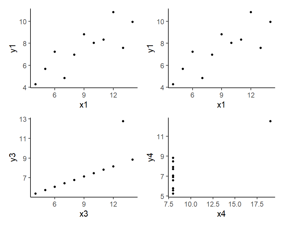

Figure 1.1: Anscombe Quartet.

In the code above, we created four separate figures, named p1, p2, p3, p4 and used the patchwork library to create a composite figure comprising the four plots. When creating the individual scatterplots, we used the pipe operator %>% to “send” the dataframe / tibble to the ggplot function, and then ‘added’ a scatterplot with the geom_point() function. The aes option (which stands for aesthetics) is used to indicate the x-variable, y-variable, color-variable, and so on. The theme_classic() function is used to create a certain “look” for the plots.

The pipe operator %>% is helpful when doing several things to a data frame in sequence, and can help create very readable code. This operator is not part of base R, but is provided by the package magrittr which is included in the dplyr package which is included in the tidyverse package.

1.6 More on the R Environment

In your Environment tab, look for the menu button marked “Global Environment” and click on the little black triangle on the right of it. You will see a large list of “environments”, most of which are packages that were loaded in your R session, either automatically or by yourself using the library() command. The “Global Environment”, which contains all the variables that you created in your session, is always first. The packages are ordered as they were loaded (latest on top). To see all the functions in a loaded package, say the package ggplot2, you can use the command ls("package:ggplot2"). Just entering ls() will list the the contents of the Global Environment.

One issue that you should pay attention to is ‘masking’. When we loaded the tidyverse package we saw two warnings: that dplyr::filter() masks stats::filter() and dplyr::lag() masks stats::lag(). Both dplyr and stats packages have a lag() function. Because the dplyr package was loaded on top of the stats package, the dplyr version ‘masks’ the stats version, and calling lag() will call the dplyr version. However, the two versions behave differently: the stats version requires the input to be a time series object, whereas the input to the dplyr version cannot be a time series object. Worse, lag(x,1) in one means something quite different from lag(x,1) in the other. We illustrate this issue in the next example. To be explicit about which version you wish to use, indicate the package using ::, as in stats::lag().

Example 1.2 In this example, we create a vector 1:10, and convert it into a time series object from 2019Q1 to 2021Q2. We then apply the dplyr version to the vector, and the stats version to the time series.

x <- 1:10
x

 [1]  1  2  3  4  5  6  7  8  9 10

lag(x,1)  # dplyr version is used

 [1] NA  1  2  3  4  5  6  7  8  9

x.ts <- ts(1:10, start=c(2019,1), frequency=4)  
x.ts

     Qtr1 Qtr2 Qtr3 Qtr4
2019    1    2    3    4
2020    5    6    7    8
2021    9   10          

stats::lag(x.ts,1)

     Qtr1 Qtr2 Qtr3 Qtr4
2018                   1
2019    2    3    4    5
2020    6    7    8    9
2021   10               

We see that the dplyr version lags the data whereas the stats version creates a “leading” series. To use the stats version to lag, we have to say stats::lag(x.ts,-1).

1.7 User-Defined Functions, Conditional Statements, Loops

You can define your own functions.

Example 1.3 A one-line function to calculate the area of a circle.

area_circle <- function(r){pi*r^2}
area_circle(2)

[1] 12.56637

Example 1.4 A more complicated function

circle_summary <- function(r=1){
  if (!is.numeric(r)){
    stop("Error: Input is not numeric.")
  } else if (r<=0 | is.nan(r) | is.infinite(r)) {
    print("Error: Please input a positive finite value for the radius.")
    return(NULL)
  } else {
    result = list("radius" = r, "area"=pi*r^2, "circumference"=2*pi*r)
    return(result)
  }
}

When the set of instructions is executed, a function object named circle_summary appears in your environment. Thereafter we can call it whenever we want to use it.

A1 = circle_summary(); A1   # radius defaults to 1

$radius
[1] 1

$area
[1] 3.141593

$circumference
[1] 6.283185

A2 = circle_summary(2); A2;

$radius
[1] 2

$area
[1] 12.56637

$circumference
[1] 12.56637

A3 = circle_summary(-1); A3

[1] "Error: Please input a positive finite value for the radius."

NULL

A4 = circle_summary("two"); A4

Error in circle_summary("two"): Error: Input is not numeric.

Error in eval(expr, envir, enclos): object 'A4' not found

The circle_summary() function requires one input r, which has the default value of 1. The function also contains “if-else” statements that carry out the following conditional actions:

• check if you put in a non-numeric value;
• if you did, print a error message and stop;
• If you did not input a non-numeric, check if it is negative or NaN or Inf;
• If so, print a different error message and return NULL (but don’t stop the program);
• If the numeric value is not negative and not NaN and not Inf, then return a list comprising the radius, area and circumference of the circle.

Blocks of code are bound with “{…}”. The way we placed the braces is somewhat conventional. Indentations and writing long commands over several lines also help with readability.

Every function call has its “own namespace”:

Example 1.5 In the following example, the assignment of the value 3 to x inside the function does not change the value of x outside of the function.

an_example_function <- function(x){
  cat("x =", x, "was passed into the function.\n")
  x <- 3;
  cat("The function changes the value to: x = ", x, ".\n", sep="")
}
x <- 1
cat("The declared value of x: x = ", x, ".\n", sep="")
an_example_function(x)
cat("The value outside the function remains unchanged: x = ", x, ".\n")

The declared value of x: x = 1.
x = 1 was passed into the function.
The function changes the value to: x = 3.
The value outside the function remains unchanged: x =  1 .

We use the function cat() to print to screen (cat == “concatenate and print”). The special code “\n” refers to a line break. The function automatically adds a space between entries. To tell the function not to add the space, set the option sep="".

Another essential programming technique is the “for-loop”. The following code, which contains a loop and a nested loop, illustrates how they work.

Example 1.6 Can you figure out what is going on in the program below?

for (A in c(TRUE,FALSE)){
  for (B in c(TRUE,FALSE)){
    cat("A is",A,"and B is",B,"then A & B is",A & B,"\n")
  }
} 

A is TRUE and B is TRUE then A & B is TRUE 
A is TRUE and B is FALSE then A & B is FALSE 
A is FALSE and B is TRUE then A & B is FALSE 
A is FALSE and B is FALSE then A & B is FALSE 

Finally, we illustrate the “while” loop:

x <- 0
while (x<10){
  cat("x = ", x, ", x < 10 is ", x<10, " so we enter the loop,\n", sep="")
  x=x+2   # this means replace current value of x with current value + 2
}
cat("x = ", x, ", x < 10 is ", x<10, " so we skip the loop.\n", sep="")

x = 0, x < 10 is TRUE so we enter the loop,
x = 2, x < 10 is TRUE so we enter the loop,
x = 4, x < 10 is TRUE so we enter the loop,
x = 6, x < 10 is TRUE so we enter the loop,
x = 8, x < 10 is TRUE so we enter the loop,
x = 10, x < 10 is FALSE so we skip the loop.

Can you see the danger of inadvertently entering an infinite loop?

Auguie, Baptiste. 2015. gridExtra: Miscellaneous Functions for "Grid" Graphics. http://CRAN.R-project.org/package=gridExtra.

Fox, John, and Sanford Weisberg. 2019. An R Companion to Applied Regression. Third. Thousand Oaks CA: Sage. https://socialsciences.mcmaster.ca/jfox/Books/Companion/.

Karline, Soetaert. 2015. plot3D. https://cran.r-project.org/web/packages/plot3D/index.html.

Meschiari, Stefano. 2023. Latex2exp: Use LaTeX Expressions in Plots.

Pedersen, Thomas Lin. 2023. Patchwork: The Composer of Plots.

Wickham, Hadley, Mara Averick, Jennifer Bryan, Winston Chang, Lucy D’Agostino McGowan, Romain François, Garrett Grolemund, et al. 2019. “Welcome to the tidyverse.” Journal of Open Source Software 4 (43): 1686. https://doi.org/10.21105/joss.01686.

Wickham, Hadley, and Jennifer Bryan. 2023. Readxl: Read Excel Files.

Zeileis, Achim, Susanne Köll, and Nathaniel Graham. 2020. “Various Versatile Variances: An Object-Oriented Implementation of Clustered Covariances in R.” J. Stat. Softw. 95 (1). https://doi.org/10.18637/jss.v095.i01.

---

1. Technically, R stores the value \(4.5\) as binary code somewhere in your computer, creates a name x, and a pointer linking the name to the memory location where the value is stored. But at this stage, you can think of it as having created an object named x with the value \(4.5\).

2. We will use the packages tidyverse (Wickham et al. (2019)) for data management and plotting, readxl (Wickham and Bryan (2023)) for importing data, car (Fox and Weisberg (2019)) and sandwich (Zeileis, Köll, and Graham (2020)) for econometrics related algorithms, and patchwork (Pedersen (2023)), latex2exp (Meschiari (2023)), gridExtra (Auguie (2015)) and plot3D (Karline (2015)) for additional plotting functionality.

3. For purposes of urban planning, Singapore’s Urban Redevelopment Authority (URA) divides the country into five regions: Central, East, North, North-East and West. These are further subdivided into 55 planning areas.