library(tidyverse)
library(readxl)
library(lmtest)
library(sandwich)
library(car)10 Instrumental Variables and Generalized Method of Moments
We present the concept of instrumental variables, and an estimation method called Generalized Method of Moments (GMM). This extended framework enables consistent estimation of economic relationships in situations where there are endogeneity problems, i.e., where (for whatever reason) there are correlations between the noise term and one or more regressors. However, it requires the availability of good instrumental variables, which may not be so easy to find.
The R code in this chapter uses the packages
We will also use Stata to verify our computations.
10.1 Instrumental Variables and the IV Estimator
Suppose the regression equation of interest is
\[
Y_i = \beta_0 + \beta_1 X_i + \epsilon_i \;,\; i=1,2,...,N.
\] We continue to assume independent observations, but suppose that \(X_i\) and \(\epsilon_i\) are correlated, with the consequence that the OLS estimator for \(\beta_1\) is inconsistent (and biased). Suppose, however, that there are observations of a third variable \(Z_i\) that are correlated with \(X_i\) but not with \(\epsilon_i\). We can use this variable to estimate \(\beta_1\) consistently.
We continue to assume that \(\epsilon_i\) is zero mean for all \(i\) (this is an innocuous assumption since the regression includes an intercept term). We therefore have the following “moment conditions” for all \(i\): \[
\begin{aligned}
E[\epsilon_{i}]
& = E[Y_{i} - \beta_0 - \beta_1 X_{i}] = 0 \\
E[\epsilon_{i}Z_{i}]
& = E[(Y_i - \beta_0 - \beta_1 X_{i})Z_{i}] = 0\,.
\end{aligned}
\tag{10.1}\] Define the “IV” estimators of \(\beta_0\) and \(\beta_1\) to be those values that solve the sample analogue of the moment conditions: \[
\begin{aligned}
(1/N)\sum_{i=1}^{N} (Y_{i} - \hat{\beta}_0^{iv} - \hat{\beta}_1^{iv} X_{i}) = 0 \\
(1/N)\sum_{i=1}^{N} (Y_{i} - \hat{\beta}_0^{iv} - \hat{\beta}_1^{iv} X_{i})Z_{i} = 0 \,.
\end{aligned}
\tag{10.2}\] This gives the estimators \[
\begin{aligned}
\hat{\beta}_0^{iv} &= \overline{Y} - \hat{\beta}_1^{iv}\overline{X} \\
\hat{\beta}_1^{iv} &= \frac{\sum_{i=1}^N(Z_i-\overline{Z})(Y_i-\overline{Y})}
{\sum_{i=1}^N(Z_i-\overline{Z})(X_i - \overline{X})}
\end{aligned}
\tag{10.3}\] which are consistent for \(\beta_0\) and \(\beta_1\) respectively. We show consistency of \(\hat{\beta}_1^{iv}\). Write \(\hat{\beta}_1^{iv}\) as
\[
\hat{\beta}_1^{iv} = \beta_1 + \frac{\sum_{i=1}^N(Z_i-\overline{Z})\epsilon_{i}}
{\sum_{i=1}^N(Z_i-\overline{Z})(X_i - \overline{X})}.
\tag{10.4}\] Dividing the numerator and denominator of the second term by \(N\) shows that it is the ratio of the sample covariance of \(Z_i\) and \(\epsilon_i\) to the sample covariance of \(Z_i\) and \(X_i\). As sample sizes increase, these sample moments converge in probability to their population counterparts. By assumption, the population covariance of \(Z_i\) and \(\epsilon_i\) is zero, whereas the population covariance of \(Z_i\) and \(X_i\) is not zero. Therefore \(\hat{\beta}_1^{iv}\) converges in probability to \(\beta_1\).
Another way to see consistency of \(\hat{\beta}_1^{iv}\) is to note that (10.1) uniquely identifies \(\beta_0\) and \(\beta_1\). Write (10.1) as \[ \begin{aligned} E[Y_i] - \beta_0 - \beta_1 E[X_i] &= 0 \\ E[Z_iY_i] - \beta_0E[Z_i] - \beta_1 E[Z_iX_i] &= 0 \,. \end{aligned} \tag{10.5}\] Solving gives \[ \begin{aligned} \beta_0 &= E[Y_i] - \beta_1 E[X_i] \\ \beta_1 &= \frac{E[Z_iY_i]-E[Z_i]E[Y_i]} {E[Z_iX_i]-E[Z_i]E[X_i]} = \frac{cov[Z_i,Y_i]}{cov[Z_i,X_i]}\;. \end{aligned} \tag{10.6}\] The solution requires \(cov[Z_i,X_i] \neq 0\), which we assume. Because the sample moments in (10.2) converge to their population counterparts, \(\hat{\beta}_0^{iv}\) and \(\hat{\beta}_1^{iv}\) converge to their population values.
Although \(\hat{\beta}_1^{iv}\) is consistent, it is biased. This is easily seen from (10.4). Taking conditional expectations does not remove the second term, since \(E[\epsilon_i | \mathrm{x},\mathrm{z}] \neq 0\).
Because \(X_i\) is correlated with \(\epsilon_i\), we say it is “endogenous” (no matter what the reason for the correlation). Because \(Z_i\) is uncorrelated with \(\epsilon_i\), we say it is “exogenous”. Because we use \(Z_i\) to identify our equation, we call it an “instrumental variable”. A valid instrumental variable, or “instrument”, is one that is exogenous but correlated with the regressor. The IV estimator is also an example of what we would call a “Method of Moments” estimator.
If \(X_{i}\) is not endogenous, then we can use it “as its own instrument”, i.e., set \(Z_{i}=X_{i}\). The sample moment conditions in (10.2) then become \[ \begin{aligned} \sum_{i=1}^{N} (Y_{i} - \hat{\beta}_0^{iv} - \hat{\beta}_1^{iv} X_{i}) = 0 \\ \sum_{i=1}^{N} (Y_{i} - \hat{\beta}_0^{iv} - \hat{\beta}_1^{iv} X_{i})X_{i} = 0 \end{aligned} \tag{10.7}\] which you will recognize as the first-order conditions for OLS estimation.
Instruments can arise from natural experiments, and incidental features of specific applications. Some examples of instruments include proximity to college, quarter of birth, and parents’ years of schooling as instruments for subject’s years of schooling; variation in state cigarette taxes for maternal smoking; Vietnam war draft lottery number for veteran status, sibling sex composition for fertility (see Angrist and Krueger (2001) for a discussion of instruments from natural experiments). They can also arise from structural characteristics of particular economic relationships. We consider a supply and demand example below.
10.2 A Simultaneous Equation Example
Suppose that the intention is to estimate the demand function for a certain good. Suppose that the market for the good can be represented by the demand and supply system: \[ \begin{aligned} Q_t^d &= \delta_0 + \delta_1 P_t + \epsilon_t^d \hspace{1cm} &(\text{Demand Eq } \delta_1 < 0) \\ Q_t^s &= \alpha_0 + \alpha_1 P_t + \epsilon_t^s \hspace{1cm} &(\text{Supply Eq } \alpha_1 > 0) \\ Q_t^s &= Q_t^d \;, \hspace{3cm} &(\text{Market Clearing}) \end{aligned} \tag{10.8}\] As discussed in Chapter 5, the observed quantities and prices occur at the intersection of the demand and supply equations. Because of this, observed prices and quantities are not representative of either the demand or supply functions.
We illustrate this phenomenon with a simulation of the case where \(\alpha_0=10\), \(\alpha_1=5\), \(\delta_0=80\) and \(\delta_1=-4\), and where the mutually independent demand and supply shocks \(\epsilon_t^d\) and \(\epsilon_t^d\) are iid \(\mathrm{Normal}(0,6)\) and \(\mathrm{Normal}(0,8)\) respectively. The demand and supply shocks lead to shifts in the demand and supply functions. We draw the demand and supply functions for 20 periods and indicate their intersection points, which are the data that we observe.
set.seed(9)
nsim <- 20
ed <- rnorm(nsim, 0, 6); es <- rnorm(nsim, 0, 8)
p <- seq(from=3,to=12,by=0.1)
a0 <- 10; a1 <- 5; b0 <- 80; b1 <- -4
plt1 <- ggplot()
for (i in 1:nsim){
  qs <- a0 + a1*p + es[i]
  qd <- b0 + b1*p + ed[i]
  peq <- (a0-b0)/(b1-a1) + (es[i]-ed[i])/(b1-a1)
  qeq <- (b0+b1*(a0-b0)/(b1-a1)) + (b1*es[i]-a1*ed[i])/(b1-a1)
  dat <- data.frame("qs"=qs, "qd"=qd, "p"=p) %>% arrange(p)
  plt1 <- plt1 +
    geom_line(data=dat, aes(y=qs,x=p), color="gray", alpha=0.4) +
    geom_line(data=dat, aes(y=qd,x=p), color="gray", alpha=0.4) +
    annotate("point", y=qeq, x=peq, size=2) + ylab("q") +
    theme_classic() + theme(axis.title.y = element_text(angle = 0))
  }; plt1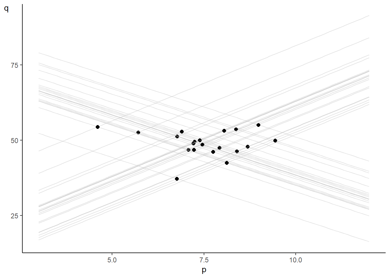
You can see that the observed prices and quantities reflect neither the demand nor the supply functions, and a regression of quantity on price will produce a slope coefficient that will turn out to be some average of \(\alpha_1\) and \(\beta_1\). The issue here is that both prices and quantity are simultaneously determined. Price, in particular, is not an exogenous variable. Variation in the data comes about because of the demand and supply shocks, both of which affect both quantities and prices. In a regression of quantity on price, the regressor (price) will be correlated with the regression noise term.
We have already demonstrated the inconsistency of the OLS estimator mathematically in chapter 5. We review the argument briefly. Solving for quantity and prices gives \[ \begin{aligned} P_t &= \frac{\alpha_0 - \delta_0}{\delta_1 - \alpha_1} + \frac{\epsilon_t^s - \epsilon_t^d}{\delta_1 - \alpha_1} \\ Q_t &= \left(\delta_0 + \delta_1\frac{\alpha_0 - \delta_0}{\delta_1 - \alpha_1}\right) + \frac{\delta_1\epsilon_t^s - \alpha_1\epsilon_t^d}{\delta_1 - \alpha_1}\,. \end{aligned} \tag{10.9}\] which implies \[ var[P_t] = \frac{\sigma_s^2 + \sigma_d^2}{(\delta_1 - \alpha_1)^2} \quad \text{ and } \quad cov[P_t, Q_t] = \frac{\delta_1\sigma_s^2 + \alpha_1\sigma_d^2}{(\delta_1 - \alpha_1)^2}. \tag{10.10}\] The OLS estimator of \(\beta_1\) in the regression \(Q_t = \beta_0 + \beta_1 P_t + \epsilon_t\) will converge to the ratio of \(cov[P_t, Q_t]\) and \(var[P_t]\): \[ \hat{\beta}_1^{ols} \rightarrow_p \frac{cov[Q_t, P_t]}{var[P_t]} =\frac{\delta_1\sigma_s^2 + \alpha_1\sigma_d^2}{\sigma_s^2 + \sigma_d^2} \] which is neither the price elasticity of demand nor the price elasticity of supply.
Suppose, however, that there is some observable variable \(r_t\) that shifts the supply function but not the demand function. That is, suppose the market for our good is represented by the equations \[ \begin{aligned} Q_t^d &= \delta_0 + \delta_1 P_t + \epsilon_t^d \hspace{1cm} &(\text{Demand Eq } \delta_1 < 0) \\ Q_t^s &= \alpha_0 + \alpha_1 P_t + \alpha_2r_t + \epsilon_t^s \hspace{0.5cm} &(\text{Supply Eq } \alpha_1 > 0) \\ Q_t^s &= Q_t^d \hspace{2.5cm} &(\text{Market Clearing}) \end{aligned} \tag{10.11}\] where \(\alpha_2 \neq 0\) and \(r_t\) is uncorrelated with the demand shocks. Because (by assumption) \(r_t\) is uncorrelated with the demand shock, and because \(r_t\) is correlated with prices (changes in \(r_t\) shift the supply function, and this changes price), it is a valid instrument. The IV estimators for \(\delta_0\) and \(\delta_1\) are then \[ \begin{aligned} \hat{\delta}_0^{iv} &= \overline{Q} - \hat{\delta}_1^{iv}\overline{P} \\ \hat{\delta}_1^{iv} &= \frac{\sum_{i=1}^T(r_t-\overline{r})(Q_t-\overline{Q})} {\sum_{i=1}^T(r_t-\overline{r})(P_t - \overline{P})}\;\;. \end{aligned} \tag{10.12}\] As argued previously, these are consistent (though biased) estimators.
10.2.1 A Two-Stage Least Squares Perspective
We continue with the demand-supply example in (10.11), and view the estimator \(\hat{\delta}_1^{iv}\) from the perspective of the following two-step procedure:
First regress the endogenous regressor \(P_t\) onto the exogenous regressor \(r_t\): \[ P_t = \phi_0 + \phi_1r_t + u_t \] and collect the fitted values \[ \hat{P}_t = \hat{\phi}_0 + \hat{\phi}_1r_t \,, \] where \[ \hat{\phi}_1 = \frac{\sum_{i=1}^T(P_t - \overline{P})(r_t-\overline{r})} {\sum_{i=1}^T(r_t-\overline{r})^2} \;. \tag{10.13}\]
Next regress \(Q_t\) on \(\hat{P}_t\) (with intercept)
Call the estimator of the coefficient on \(\hat{P}_t\) in this regression \(\hat{\delta}_1^{2sls}\) where “2sls” stands for “2-Stage Least Squares”. We have \[
\hat{\delta}_1^{2sls} = \frac{\sum_{i=1}^T(Q_t - \overline{Q})(\hat{P}_t-\overline{\hat{P}})}{\sum_{i=1}^T(\hat{P}_t - \overline{\hat{P}})^2} \;.
\tag{10.14}\] This estimator turns out to be identical to \(\hat{\delta}_1^{iv}\). Since \(\hat{P}_t = \hat{\phi}_0 + \hat{\phi}_1r_t\), we have \[
\hat{P}_t - \overline{\hat{P}} = \hat{\phi}_1 (r_t - \overline{r}) \;,
\tag{10.15}\] therefore \[
\hat{\delta}_1^{2sls} =
\frac{\hat{\phi}_1\sum_{i=1}^T(Q_t-\overline{Q})(r_t-\overline{r})}
{\sum_{i=1}^T(\hat{P}_t - \overline{\hat{P}})^2} \;.
\] Summing (10.15) over all observations gives
\[
\sum_{i=1}^T(\hat{P}_t - \overline{\hat{P}})^2
= \hat{\phi}_1^2 \sum_{t=1}^T(r_t - \overline{r})^2
= \hat{\phi}_1 \sum_{i=1}^T(P_t - \overline{P})(r_t-\overline{r})
\] where we used the expression (10.13) for \(\hat{\phi}_{1}\). It follows that \[
\hat{\delta}_1^{2sls}
=
\frac{\sum_{i=1}^T(Q_t-\overline{Q})(r_t-\overline{r})}
{\sum_{i=1}^T(P_t - \overline{P})(r_t-\overline{r})}
\] which is the same expression as \(\hat{\delta}_1^{iv}\).
The intuition is as follows. Imagine that we can “shut down” the supply and demand shocks. Then the demand function does not shift, whereas the supply function shifts as \(r_t\) varies. The intersection points then map out the demand function, as illustrated below:
r <- rnorm(nsim, 2, 3)
a2 <- 4
plt2 <- ggplot()
for (i in 1:nsim){
  qs <- a0 + a1*p + a2*r[i]
  qd <- b0 + b1*p
  peq <- (a0-b0)/(b1-a1) + a2*r[i]/(b1-a1)
  qeq <- (b0+b1*(a0-b0)/(b1-a1)) + b1*a2*r[i]/(b1-a1)
  dat <- data.frame("qs"=qs, "qd"=qd, "p"=p) %>% arrange(p)
  plt2 <- plt2 +
    geom_line(data=dat, aes(y=qs,x=p), color="gray", alpha=0.4) +
    geom_line(data=dat, aes(y=qd,x=p), color="gray", alpha=0.4) +
    annotate("point", y=qeq, x=peq, size=2) +
    theme_minimal()
  }
plt2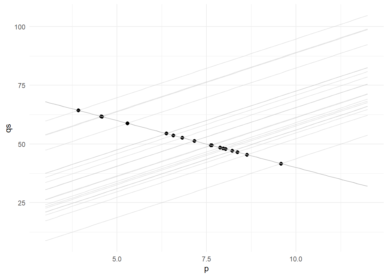
In other words, movements in \(r_t\) can help to ‘trace out’ the demand function. The problem, however, is that the “real data” also contains movements due to the demand and supply shocks. We get around this problem by isolating movements in \(P_t\) that are due to solely to movements in \(r_t\). This is done in the first stage regression where we regress \(P_t\) on \(r_t\). Since the fitted values \(\hat{P}_t\) is equal to \(\hat{\phi}_0 + \hat{\phi}_1r_t\), and \(r_t\) is exogenous, so is \(\hat{P}_t\). We get a consistent estimator of \(\delta_1\) by regressing \(Q_t\) on \(\hat{P}_t\), i.e., by employing only that part of \(P_t\) that is uncorrelated with the demand and supply shocks.
Although IV estimation gives consistent estimators despite the presence of endogenous regressors, it does so at a cost. Since \(\hat{\delta}_1^{iv}\) is, in essence, obtained from a regression of \(Q_t\) on \(\hat{P}_t\), and because there is less variation in \(\hat{P}_t\) than in \(P_t\) (why?), there is a reduction in effective variation in the regressor. This results in an increase in the variance of the estimator as compared to if we had regressed \(Q_t\) on \(P_t\). If \(P_t\) is endogenous, then this would seem to be a good tradeoff, since the alternative is an inconsistent estimator. However, if the correlation between \(P_t\) and \(r_t\) is weak, the reduction in effective variation will be substantial, and this will result in very imprecise estimators. This loss of precision has to be weighed against the perceived degree of endogeneity in the regressor.
IV estimators can behave very poorly if instruments are not valid (in the sense of being poorly correlated with the endogenous regressors) and if there is some degree of endogeneity. We can get some intuition for why IV estimators are likely to perform poorly in these circumstances by referring to Eq. 10.4.
10.3 Multiple Instruments
We discuss situations where we have multiple endogenous regressor and multiple instruments. We revert to generic notation for our regressions, and continue to assume a sample of independent draws of size \(N\) throughout. We first note that having exogenous and endogenous regressors in the regression at the same time does not present any particular difficulty.
Suppose the regression equation of interest is: \[ Y_i = \beta_0 + \beta_1 X_{1,i} + \beta_1 X_{2,i} + \epsilon_i \] where \(X_{1,i}\) is an exogenous regressor (not correlated with the noise term) and \(X_{2,i}\) is an endogenous regressor (correlated with the noise term). Suppose there is a variable \(Z_{1,i}\) that is correlated with \(X_{2,i}\) and uncorrelated with the noise term. Then we have the moment conditions \[ \begin{aligned} E[\epsilon_{i}] & = E[Y_{i} - \beta_0 - \beta_1 X_{1,i} - \beta_2 X_{2,i}] = 0 \\[2ex] E[\epsilon_{i}X_{1,i}] & = E[(Y_i - \beta_0 - \beta_1 X_{1,i} - \beta_2 X_{2,i})X_{1,i}] = 0 \\[2ex] E[\epsilon_{i}Z_{1,i}] & = E[(Y_i - \beta_0 - \beta_1 X_{1,i} - \beta_2 X_{2,i})Z_{1,i}] = 0 \,. \end{aligned} \tag{10.16}\] The sample analogue of (10.16) is \[ \begin{aligned} \sum_{i=1}^{N} (Y_{i} - \hat{\beta}_0^{iv} - \hat{\beta}_1^{iv} X_{1,i} - \hat{\beta}_2^{iv} X_{2,i}) = 0 \\ \sum_{i=1}^{N} (Y_{i} - \hat{\beta}_0^{iv} - \hat{\beta}_1^{iv} X_{1,i} - \hat{\beta}_2^{iv} X_{2,i})X_{1,i}= 0 \\ \sum_{i=1}^{N} (Y_{i} - \hat{\beta}_0^{iv} - \hat{\beta}_1^{iv} X_{1,i} - \hat{\beta}_2^{iv} X_{2,i})Z_{1,i}= 0 \,. \end{aligned} \tag{10.17}\] The IV estimators are those values \(\hat{\beta}_{0}^{iv}\), \(\hat{\beta}_{1}^{iv}\) and \(\hat{\beta}_{2}^{iv}\) that solve (10.17). Of course, not all three-equation systems in three unknowns can be solved. The condition that \(Z_{1,i}\) be correlated with the endogenous regressor is required for the system to be solvable.
What if we have more than one instrument? Suppose we have \(Z_{1,i}\) and \(Z_{2,i}\) that are not correlated with the regression noise term, but correlated with the endogenous regressor? (Imagine that there are two exogenous variables that shift the only supply function in our demand-supply example.) In this case we have more moment equations than parameters:
\[
\begin{aligned}
E[\epsilon_{i}]
& = E[Y_{i} - \beta_0 - \beta_1 X_{1,i}
- \beta_2 X_{2,i}] = 0 \\[2ex]
E[\epsilon_{i}X_{1,i}]
& = E[(Y_i - \beta_0 - \beta_1 X_{1,i}
- \beta_2 X_{2,i})X_{1,i}] = 0 \\[2ex]
E[\epsilon_{i}Z_{2,i}]
& = E[(Y_i - \beta_0 - \beta_1 X_{1,i}
- \beta_2 X_{2,i})Z_{1,i}] = 0 \\[2ex]
E[\epsilon_{i}Z_{3,i}]
& = E[(Y_i - \beta_0 - \beta_1 X_{1,i}
- \beta_2 X_{2,i})Z_{2,i}] = 0 \,.
\end{aligned}
\tag{10.18}\] The sample analogues of the moment conditions are: \[
\begin{aligned}
\sum_{i=1}^{N} (Y_{i} - \hat{\beta}_0 - \hat{\beta}_1 X_{1,i}
- \hat{\beta}_2 X_{2,i}) = 0 \\
\sum_{i=1}^{N} (Y_{i} - \hat{\beta}_0 - \hat{\beta}_1 X_{1,i}
- \hat{\beta}_2 X_{2,i})X_{1,i}= 0 \\
\sum_{i=1}^{N} (Y_{i} - \hat{\beta}_0 - \hat{\beta}_1 X_{1,i}
- \hat{\beta}_2 X_{2,i})Z_{1,i}= 0 \\
\sum_{i=1}^{N} (Y_{i} - \hat{\beta}_0 - \hat{\beta}_1 X_{1,i}
- \hat{\beta}_2 X_{2,i})Z_{2,i}= 0 \,.
\end{aligned}
\tag{10.19}\] We cannot solve four moment conditions for three parameters, unless the moment conditions are dependent. However, we can set \(\hat{\beta}_{0}\), \(\hat{\beta}_{1}\) and \(\hat{\beta}_{2}\) so that the values on the left hand side of the equations in (10.19) are as close to zero as possible, in some sense. For instance, we can set \(\hat{\beta}_{0}\), \(\hat{\beta}_{1}\) and \(\hat{\beta}_{2}\) so that the sum of the square of the four values on the LHS of (10.19) are minimized. We will label these estimators “MM” (for “Method of Moments”).
At this point, it is easier to switch to matrix algebra. Write \[ y = \begin{bmatrix} Y_1 \\ Y_2 \\ \vdots \\ Y_N \end{bmatrix}\, , \; X = \begin{bmatrix} 1 & X_{1,1} & X_{2,1} \\ 1 & X_{1,2} & X_{2,2} \\ \vdots & \vdots & \vdots \\ 1 & X_{1,N} & X_{2,N} \\ \end{bmatrix}\, , \; \varepsilon = \begin{bmatrix} \epsilon_1 \\ \epsilon_2 \\ \vdots \\ \epsilon_N \end{bmatrix}\, , \; Z = \begin{bmatrix} 1 & X_{1,1} & Z_{1,1} & Z_{2,1}\\ 1 & X_{1,2} & Z_{1,2} & Z_{2,2}\\ \vdots & \vdots & \vdots &\vdots \\ 1 & X_{1,N} & Z_{1,N} & Z_{2,N}\\ \end{bmatrix} \;. \] Let \(x_i^\mathrm{T} = \begin{bmatrix}1 & X_{1,i} & X_{2,i} \end{bmatrix}\) and \(z_i^\mathrm{T} = \begin{bmatrix} 1 & X_{1,i} & Z_{1,i} & Z_{2,i} \end{bmatrix}\). The regression equation is then \[ y = X\beta + \varepsilon \] or \[ Y_i = x_{i}^{\mathrm{T}}\beta + \epsilon_i\,,i=1,2,...,N, \] and where \[ \beta = \begin{bmatrix} \beta_0 \\ \beta_1 \\ \beta_2 \end{bmatrix} \,. \] The population moment conditions in (10.18) can be written as \[ E[z_i(Y_i-\beta_0 - x_{i}^{\mathrm{T}}\beta_1)] = E[z_i\epsilon_i] = 0 \,. \] The sample analogue (10.19) can be written as \[ Z^\mathrm{T}(y-X\hat{\beta}^{mm}) = Z^\mathrm{T}y-Z^\mathrm{T}X\hat{\beta}^{mm} = 0 \;. \] The “Sum of Squared Moments” is then \[ (Z^\mathrm{T}y-Z^\mathrm{T}X\hat{\beta}^{mm})^\mathrm{T}(Z^\mathrm{T}y-Z^\mathrm{T}X\hat{\beta}^{mm})\,. \tag{10.20}\] Minimizing (10.20), we get \[ \hat{\beta}^{mm} = (X^\mathrm{T}ZZ^\mathrm{T}X)^{-1}X^\mathrm{T}ZZ^\mathrm{T}y \tag{10.21}\] (see exercises) where we assume that \(X^\mathrm{T}ZZ^\mathrm{T}X\) is invertible. We can also write \(\hat{\beta}^{mm}\) as \[ \begin{aligned} \hat{\beta}^{mm} &= (X^\mathrm{T}ZZ^\mathrm{T}X)^{-1}X^\mathrm{T}ZZ^\mathrm{T}(X\beta + \varepsilon) \\ &= \beta + (X^\mathrm{T}ZZ^\mathrm{T}X)^{-1}X^\mathrm{T}ZZ^\mathrm{T}\varepsilon \\ &= \beta + \left[(\tfrac{1}{N}X^\mathrm{T}Z)(\tfrac{1}{N}Z^\mathrm{T}X)\right]^{-1}(\tfrac{1}{N}X^\mathrm{T}Z)(\tfrac{1}{N}Z^\mathrm{T}\varepsilon). \end{aligned} \] Note that \[ \tfrac{1}{N}X^\mathrm{T}Z = \tfrac{1}{N}\sum_{i=1}^N x_i z_i^\mathrm{T} \,,\; \tfrac{1}{N}Z^\mathrm{T}\varepsilon = \tfrac{1}{N}\sum_{i=1}^N z_i \epsilon_i \,,\; \text{etc.} \] Roughly speaking, \(\hat{\beta}^{mm}\) will be consistent if the sample covariances in \(\tfrac{1}{N}\sum_{i=1}^N z_i \epsilon_i\) converge in probability to their population counterparts, which are zero if the instruments (the variables in \(Z\)) are exogenous. As with the IV estimator, the MM estimator described here is biased. Taking conditional expectations (given \(X\) and \(Z\)) of \(\hat{\beta}^{mm}\) does not remove the term \((X^\mathrm{T}ZZ^\mathrm{T}X)^{-1}X^\mathrm{T}ZZ^\mathrm{T}\varepsilon\), as we do not have \(E[\varepsilon|X,Z]=0\).
If there are as many variables in \(Z\) as there are in \(X\) (i.e., if we have as many instruments as endogenous regressors), then \(X^\mathrm{T}Z\) is square, and assuming that \(X^\mathrm{T}Z\) is invertible, (10.21) reduces to \[ \hat{\beta}^{iv} = (Z^\mathrm{T}X)^{-1}Z^\mathrm{T}y \tag{10.22}\] which we refer to as the IV estimator, cf. (10.3).
What if take a two-stage least squares approach? (And how would we do it?) The first stage regression would be:
Regress each endogenous regressor on all of the exogenous variables (exogenous regressors and instruments). In the context of our specific example (one exogenous regressor \(X_{1,i}\), one endogenous regressor \(X_{2,i}\), and two instruments \(Z_{1,i}\) and \(Z_{2,i}\)), this would mean regressing \(X_{2,i}\) on a constant, \(X_{1,i}\), \(Z_{1,i}\) and \(Z_{2,i}\), and computing the fitted values \[ \hat{X}_{2,i} = \hat{\phi_0} + \hat{\phi_1}X_{1,i} + \hat{\phi_2}Z_{1,i} + \hat{\phi_3}Z_{2,i}. \]
In the second step, replace the endogenous regressors with the fitted endogenous regressors \[ Y_i = \beta_0 + \beta_1 X_{1,i} + \beta_1 \hat{X}_{2,i} + u_i \] and estimate by OLS to get the 2SLS estimators \(\hat{\beta}_0^{2sls}\), \(\hat{\beta}_1^{2sls}\) and \(\hat{\beta}_2^{2sls}\).
We can write the two steps above using matrix algebra as follows. In the first step, we regress \(X\) on \(Z\) to get the estimator \(\hat{B} = (Z^\mathrm{T}Z)^{-1}Z^\mathrm{T}X\). The fitted values are then \(\hat{X} = Z\hat{B} = Z(Z^\mathrm{T}Z)^{-1}Z^\mathrm{T}X\). These might seem like odd statements since \(X\) contains three columns: recall that \[ X = \begin{bmatrix} 1 & X_{1,1} & X_{2,1} \\ 1 & X_{1,2} & X_{2,2} \\ \vdots & \vdots & \vdots \\ 1 & X_{1,N} & X_{2,N} \\ \end{bmatrix}\, \text{ and } \; Z = \begin{bmatrix} 1 & X_{1,1} & Z_{1,1} & Z_{2,1}\\ 1 & X_{1,2} & Z_{1,2} & Z_{2,2}\\ \vdots & \vdots & \vdots &\vdots \\ 1 & X_{1,N} & Z_{1,N} & Z_{2,N}\\ \end{bmatrix} \,. \] Regressing \(X\) on \(Z\) means regressing each column of \(X\) on \(Z\), and the columns of \(\hat{B}\) contain the estimators from each of these regressions. Likewise, the columns of the fitted matrix \(\hat{X}\) contain the fitted values from each of the regressions. Regressing a column of ones on \(Z\) simply returns the column of ones as the fitted values (think about it). Regressing the column of \(X_{1,i}\) observations on \(Z\) will likewise simply return the column of \(X_{1,i}\) observations. Regressing the column of \(X_{2,i}\) observations on \(Z\) is exactly the first stage regression that we described earlier.
In the second step, we regress \(y\) on \(\hat{X}\) to get the 2SLS estimator \[ \begin{aligned} \hat{\beta}^{2sls} &= (\hat{X}^\mathrm{T}\hat{X})^{-1}\hat{X}^\mathrm{T}y \\ &= (X^\mathrm{T}Z(Z^\mathrm{T}Z)^{-1}Z^\mathrm{T}Z(Z^\mathrm{T}Z)^{-1}Z^\mathrm{T}X)^{-1} X^\mathrm{T}Z(Z^\mathrm{T}Z)^{-1}Z^\mathrm{T}y \\ &= (X^\mathrm{T}Z(Z^\mathrm{T}Z)^{-1}Z^\mathrm{T}X)^{-1} X^\mathrm{T}Z(Z^\mathrm{T}Z)^{-1}Z^\mathrm{T}y \;. \end{aligned} \tag{10.23}\] The 2SLS estimator (10.23) and what we have called the MM estimator are different, but both are consistent. It is easy to show that if \(X\) and \(Z\) have the same number of columns (so \(X^\mathrm{T}Z\) is square) then they both reduce to what we have called the IV estimator.
The formulas derived extend without change to the case where there are \(K\) exogenous regressors (in addition to the constant), \(G\) endogenous regressors, and \(M\) instrumental variables, where \(M \geq G\). That is, suppose we are interested in estimating the regression \[ \begin{aligned} Y_i &= \beta_0 + \beta_1 X_{1,i}^k + \dots \beta_{K} X_{K,i}^k + \beta_{K+1}X_{K+1,i}^g + \dots + \beta_{K+G}X_{K+G,i}^g + \epsilon_i \\ &= x_i^\mathrm{T}\beta + \epsilon_i \end{aligned} \] where we use the \(k\) and \(g\) superscripts to denote the exogenous and endogenous regressors, and the \(K+G+1\) vector \(x_i\) is \[ x_i^\mathrm{T} = \begin{bmatrix} 1 & X_{1,i}^k & \dots & X_{K,i}^k & X_{K+1,i}^g & \dots & X_{K+G,i}^g \end{bmatrix}. \] Suppose you are able to find \(M \geq G\) instruments \(Z_{1,i}\), \(Z_{2,i}\), \(\dots\), \(Z_{M_i}\). Define the \(K+M+1\) vector \(z_i\) as \[ z_i^\mathrm{T} = \begin{bmatrix} 1 & X_{1,i}^k & \dots & X_{K,i}^k & Z_{1,i} & \dots & Z_{M,i} \end{bmatrix}. \] Let \[ X = \begin{bmatrix} x_1^\mathrm{T} \\ x_2^\mathrm{T} \\ \vdots \\ x_N^\mathrm{T} \end{bmatrix} \; \text{ and } \; Z = \begin{bmatrix} z_1^\mathrm{T} \\ z_2^\mathrm{T} \\ \vdots \\ z_N^\mathrm{T} \end{bmatrix}. \] Then the formulas (10.21), (10.22) and (10.23) for the “Method of Moments”, IV and 2SLS estimators all continue to apply. The inverses in those formulas must exist, of course. This requires that the instruments be correlated with the endogenous variables, and also that \(M \geq G\). If \(M=G\), then the formulas all reduce to the IV estimator. If \(Z=X\), then the IV estimator is simply the OLS estimator. If \(M=G\), we say that the regression is just identified. If \(M > G\), we say that the regression is over-identified.
10.4 Generalized Method of Moments
Finally we define the GMM estimator as those that minimize a weighted sum of squared moments, i.e.,
\[
\hat{\beta}_{W}^{gmm}
= \text{argmin}_{\hat{\beta}} \;J(W_N)
\] where \[
\begin{aligned}
J(W_N) &= (Z^\mathrm{T}y-Z^\mathrm{T}X\hat{\beta})^\mathrm{T}
W_N (Z^\mathrm{T}y-Z^\mathrm{T}X\hat{\beta}) \\
&= y^\mathrm{T}ZZ^\mathrm{T}y
- 2\hat{\beta}^\mathrm{T}X^\mathrm{T}ZW_NZ^\mathrm{T}y
+ \hat{\beta}^\mathrm{T}X^\mathrm{T}ZW_NZ^\mathrm{T}X\hat{\beta}
\end{aligned}
\tag{10.24}\] and where \(W_N\) is a symmetric positive-definite matrix of “weights” (the weights may be data dependent). The resulting estimator depends on the choice of weights, which is the reason for the subscript \(W\) in \(\hat{\beta}_{W}^{gmm}\). Minimizing (10.24), we get \[
\hat{\beta}_{W}^{gmm} = (X^\mathrm{T}ZW_NZ^\mathrm{T}X)^{-1}X^\mathrm{T}ZW_NZ^\mathrm{T}y \;.
\tag{10.25}\] To derive the properties of this estimator, we make the following assumptions:
Assumption Set F:
(F1) The equation to be estimated is \[ Y_i = x_i^\mathrm{T}\beta + \epsilon_i \;,\; i=1,2,...,N \] where \(x_i\) is the vector \[ x_i^\mathrm{T} = \begin{bmatrix} 1 & X_{1,i}^k & \dots & X_{K,i}^k & X_{K+1,i}^g & \dots & X_{K+G,i}^g \end{bmatrix} \] and where \(X_{1,i}^{k}\),…, \(X_{K,i}^{k}\) are \(K\) variables known to be exogenous, and \(X_{K+1,i}^g\),…, \(X_{K+G,i}^{g}\) are \(G\) variables thought to be endogenous.
(F2) There are \(M\) instruments \(Z_{1,i}\), …, \(Z_{M,i}\) such that the vector \(z_i\) defined as \[ z_i^\mathrm{T} = \begin{bmatrix} 1 & X_{1,i}^k & \dots & X_{K,i}^k & Z_{1,i} & \dots & Z_{M,i} \end{bmatrix} \] has the following properties:
(F3) the \(((K+M+1) \times (K+G+1))\) matrix \(E[z_ix_i^\mathrm{T}] = \Sigma_{zx}\) has full column rank,
(F4) \(E[\epsilon_i|z_i] = 0\),
(F5) \(E[\epsilon_i^2z_{i}z_{i}^\mathrm{T}] = S\) is finite and non-singular.
Furthermore, assume
(F6) the unique random variables in \(\{x_i,z_i\}\) are i.i.d., and
(F7) \(W_N\) is chosen such that \(W_N \rightarrow_p W\) symmetric and positive-definite.
Let \(X\) and \(Z\) be as previously defined. The estimator (10.25) is consistent: \[ \begin{aligned} \hat{\beta}_{W}^{gmm} &= (X^\mathrm{T}ZW_NZ^\mathrm{T}X)^{-1}X^\mathrm{T}ZW_NZ^\mathrm{T}y \\ &= \beta + (X^\mathrm{T}ZW_NZ^\mathrm{T}X)^{-1}X^\mathrm{T}ZW_NZ^\mathrm{T}\varepsilon \\ &= \beta + [(\tfrac{1}{N}X^\mathrm{T}Z)W_N(\tfrac{1}{N}Z^\mathrm{T}X)]^{-1}(\tfrac{1}{N}X^\mathrm{T}Z)W_N(\tfrac{1}{N}Z^\mathrm{T}\varepsilon) \\ &\rightarrow_p \beta + (\Sigma_{zx}^\mathrm{T}W\Sigma_{zx})^{-1}\Sigma_{zx}^\mathrm{T}W0 \\ &= \beta \end{aligned} \] since under our assumptions \[ \frac{1}{N}Z^\mathrm{T}X = \frac{1}{N} \sum_{i=1}^Nz_ix_i^\mathrm{T} \rightarrow_p \Sigma_{zx} \] and \[ \frac{1}{N}Z^\mathrm{T}\epsilon = \frac{1}{N} \sum_{i=1}^Nz_i\epsilon_i \rightarrow_p 0. \] Furthermore, \[ \begin{aligned} \sqrt{N}(\hat{\beta}_{W}^{gmm} - \beta) &= [(\tfrac{1}{N}X^\mathrm{T}Z)W_N(\tfrac{1}{N}Z^\mathrm{T}X)]^{-1}(\tfrac{1}{N}X^\mathrm{T}Z)W_N(\tfrac{1}{\sqrt{N}}Z^\mathrm{T}\varepsilon) \\ &\rightarrow_d \mathrm{Normal}(0, (\Sigma_{zx}^\mathrm{T}W\Sigma_{zx})^{-1} \Sigma_{zx}^\mathrm{T}WSW\Sigma_{zx} (\Sigma_{zx}^\mathrm{T}W\Sigma_{zx})^{-1}) \end{aligned} \] since under our assumptions, \[ \frac{1}{\sqrt{N}}Z^\mathrm{T}\varepsilon \rightarrow_d \mathrm{Normal}(0,S)\;. \] The asymptotic variance of the GMM estimator is \[ \mathrm{avar}[\hat{\beta}_{W}^{gmm}] = (\Sigma_{zx}^\mathrm{T}W\Sigma_{zx})^{-1} \Sigma_{zx}^\mathrm{T}WSW\Sigma_{zx} (\Sigma_{zx}^\mathrm{T}W\Sigma_{zx})^{-1}\;. \tag{10.26}\] We approximate the finite sample variance of \(\hat{\beta}_{W}^{gmm}\) by \[ var[\hat{\beta}_{W}^{gmm}] \approx \frac{1}{N} (\Sigma_{zx}^\mathrm{T}W\Sigma_{zx})^{-1} \Sigma_{zx}^\mathrm{T}WSW\Sigma_{zx} (\Sigma_{zx}^\mathrm{T}W\Sigma_{zx})^{-1}) \] To operationalize this estimator, we need to estimate the various elements in the formula for \(var[\hat{\beta}_{W}^{gmm}]\). Assume for the moment that we know \(W\). For \(\Sigma_{zx}\) we can use \[ \hat{\Sigma}_{zx} = \frac{1}{N}\sum_{i=1}^Nz_{i}x_{i}^\mathrm{T}=\frac{1}{N}Z^\mathrm{T}X. \] For \(S\) we can use \[ \hat{S} = \frac{1}{N}\sum_{i=1}^N \hat{\epsilon}_i^2 z_i z_i^\mathrm{T}. \] In other words, we can estimate the variance of \(\hat{\beta}_{W}^{gmm}\) with \[ \begin{aligned} \widehat{var}[\hat{\beta}_{W}^{gmm}] &= \frac{1}{N} (\hat{\Sigma}_{zx}^\mathrm{T}W\hat{\Sigma}_{zx})^{-1} \hat{\Sigma}_{zx}^\mathrm{T}W\hat{S}W\hat{\Sigma}_{zx} (\hat{\Sigma}_{zx}^\mathrm{T}W\hat{\Sigma}_{zx})^{-1} \\ &= (X^\mathrm{T}ZWZ^\mathrm{T}X)^{-1} X^\mathrm{T}ZW \left[ \sum_{i=1}^N \hat{\epsilon}_i^2 z_i z_i^\mathrm{T}\right] WZ^\mathrm{T}X (X^\mathrm{T}ZWZ^\mathrm{T}X)^{-1} \end{aligned} \tag{10.27}\] This variance estimator is heteroskedasticity-robust.
Remarks:
In the just-identified case, the GMM estimator reduces to the IV estimator regardless of \(W_N\): \[ \begin{aligned} \hat{\beta}_{W}^{gmm} &= (X^\mathrm{T}ZW_NZ^\mathrm{T}X)^{-1}X^\mathrm{T}ZW_NZ^\mathrm{T}y\; \\ &= (Z^\mathrm{T}X)^{-1}Z^\mathrm{T}y \\ &= \hat{\beta}^{iv} \,. \end{aligned} \tag{10.28}\] The asymptotic variance (10.26) becomes \[ \mathrm{avar}[\hat{\beta}^{iv}] = \Sigma_{zx}^{-1}S(\Sigma_{zx}^\mathrm{T})^{-1} \,. \] The variance estimator (10.27) becomes \[ \widehat{var}[\hat{\beta}^{iv}] = (Z^\mathrm{T}X)^{-1} \left[ \sum_{i=1}^N \hat{\epsilon}_i^2 z_i z_i^\mathrm{T}\right] (X^\mathrm{T}Z)^{-1}\;. \]
If we choose \(W_N = I\), the identity matrix, then \[ \begin{aligned} \hat{\beta}_{I}^{gmm} &= (X^\mathrm{T}ZW_NZ^\mathrm{T}X)^{-1}X^\mathrm{T}ZW_NZ^\mathrm{T}y \\ &= (X^\mathrm{T}ZZ^\mathrm{T}X)^{-1}X^\mathrm{T}ZZ^\mathrm{T}y \\ &= \hat{\beta}^{mm}, \\ \end{aligned} \] the “MM” estimator presented earlier. The variance estimator (10.27) becomes \[ \widehat{var}[\hat{\beta}^{mm}] = (X^\mathrm{T}ZZ^\mathrm{T}X)^{-1} X^\mathrm{T}Z \left[ \sum_{i=1}^N \hat{\epsilon}_i^2 z_i z_i^\mathrm{T}\right] Z^\mathrm{T}X (X^\mathrm{T}ZZ^\mathrm{T}X)^{-1}\,. \tag{10.29}\]
If we choose \(W_N = ((1/N)Z^\mathrm{T}Z)^{-1}\), then the GMM estimator becomes the 2SLS estimator: \[ \begin{aligned} \hat{\beta}_{(Z^\mathrm{T}Z)^{-1}}^{gmm} &= (X^\mathrm{T}ZW_NZ^\mathrm{T}X)^{-1}X^\mathrm{T}ZW_NZ^\mathrm{T}y \\ &= (X^\mathrm{T}Z(Z^\mathrm{T}Z)^{-1}Z^\mathrm{T}X)^{-1}X^\mathrm{T}Z(Z^\mathrm{T}Z)^{-1}Z^\mathrm{T}y \\ &= \hat{\beta}^{2sls}. \end{aligned} \] Since \([(1/N)Z^\mathrm{T}Z]^{-1} \rightarrow_p \Sigma_{zz}^{-1}\), the asymptotic variance of the GMM estimator becomes \[ \mathrm{avar}[\hat{\beta}^{2sls}] = (\Sigma_{zx}^\mathrm{T}\Sigma_{zz}^{-1}\Sigma_{zx})^{-1} \Sigma_{zx}^\mathrm{T}\Sigma_{zz}^{-1}S\Sigma_{zz}^{-1}\Sigma_{zx} (\Sigma_{zx}^\mathrm{T}\Sigma_{zz}^{-1}\Sigma_{zx})^{-1}\;. \tag{10.30}\] where \(\Sigma_{zz}=E[z_iz_i^\mathrm{T}]\).
Note that expression (10.30) allows for conditional heteroskedasticity, but if there is conditional homoskedasticity, then \[ S = E[\epsilon_i^2 z_iz_i^\mathrm{T}] = E[E[\epsilon_i^2 z_iz_i^\mathrm{T}|z_i]] = E[E[\epsilon_i^2 |z_i]z_iz_i^\mathrm{T}] = \sigma^2E[z_iz_i^\mathrm{T}]] = \sigma^2\Sigma_{zz} \] and the asymptotic variance reduces to \[ \mathrm{avar}[\hat{\beta}^{2sls}] = \sigma^2(\Sigma_{zx}^\mathrm{T}\Sigma_{zz}^{-1}\Sigma_{zx})^{-1} \;. \tag{10.31}\] We can estimate the estimator variance by \[ \widehat{var}[\hat{\beta}^{2sls}] = \widehat{\sigma^2}(X^\mathrm{T}Z(Z^\mathrm{T}Z)^{-1}Z^\mathrm{T}X)^{-1}. \] where \(\widehat{\sigma^2}\) is some consistent estimator for \(\sigma^2\).
10.4.1 Optimal GMM
It turns out that the (asymptotically) optimal weight is to choose \(W_N\) such that \(W_N \rightarrow_p S^{-1}\). This is because the asymptotic variance of \(\hat{\beta}^{gmm}\) then becomes \[ \begin{aligned} \mathrm{avar}[\hat{\beta}^{gmm}] &= (\Sigma_{zx}^\mathrm{T}W\Sigma_{zx})^{-1} \Sigma_{zx}^\mathrm{T}WSW\Sigma_{zx} (\Sigma_{zx}^\mathrm{T}W\Sigma_{zx})^{-1}) \\ &= (\Sigma_{zx}^\mathrm{T}S^{-1}\Sigma_{zx})^{-1} \end{aligned} \] and it can be shown that \[ (\Sigma_{zx}^\mathrm{T}W\Sigma_{zx})^{-1} \Sigma_{zx}^\mathrm{T}WSW\Sigma_{zx} (\Sigma_{zx}^\mathrm{T}W\Sigma_{zx})^{-1}) -(\Sigma_{zx}^\mathrm{T}S^{-1}\Sigma_{zx})^{-1} \tag{10.32}\] is positive definite for any symmetric positive definite \(W\). A natural weight matrix to choose is therefore \[ W_N = \hat{S}^{-1} = \left[\frac{1}{N}\sum_{i=1}^N \hat{\epsilon_i}^2 z_{i} z_{i}^\mathrm{T}\right]^{-1}. \] The problem with this is that we need to have the residuals \(\hat{\epsilon}_i\) in order to compute \(\hat{S}^{-1}\), but we need an estimator of \(\beta\) in order to compute the residuals. One solution is to take a two-step approach:
- Compute \(\hat{\beta}_{W}^{gmm}\) for some (non-optimal) weighting matrix \(W_N\). A common choice is to use \(W_N = ((1/N)Z^\mathrm{T}Z)^{-1}\), which gives the (inefficient but consistent) 2SLS estimator \(\hat{\beta}^{2sls}\). Then calculate \(\hat{S}^{-1}\) using the residuals \[ \hat{\epsilon}_i = Y_i - x_i^{\mathrm{T}}\hat{\beta}^{2sls}\,. \]
- Calculate the optimal GMM estimator as \[ \hat{\beta}^{gmm} = (X^\mathrm{T}Z\hat{S}^{-1}Z^\mathrm{T}X)^{-1}X^\mathrm{T}Z\hat{S}^{-1}Z^\mathrm{T}y. \] The asymptotic variance of the Optimal GMM estimator is \[ \mathrm{avar}[\hat{\beta}^{gmm}] = (\Sigma_{zx}^\mathrm{T}S^{-1}\Sigma_{zx})^{-1}\;. \tag{10.33}\] The variance estimator becomes \[ \begin{aligned} \widehat{var}[\hat{\beta}^{gmm}] &= \frac{1}{N} \left\{\left( \frac{1}{N} \sum_{i=1}^N z_ix_i^\mathrm{T}\right)^\mathrm{T} \left[\frac{1}{N}\sum_{i=1}^N \hat{\epsilon_i}^2 z_{i} z_{i}^\mathrm{T}\right]^{-1} \left( \frac{1}{N} \sum_{i=1}^N z_ix_i^\mathrm{T}\right)\right\}^{-1} \\ &= \left\{X^\mathrm{T}Z\left[\sum_{i=1}^N \hat{\epsilon_i}^2 z_{i} z_{i}^\mathrm{T}\right]^{-1}Z^\mathrm{T}X\right\}^{-1}. \end{aligned} \tag{10.34}\]
Notice that the asymptotic variance of the optimal GMM estimator under conditional homoskedasticity becomes \[ \mathrm{avar}[\hat{\beta}^{gmm}] = \sigma^2(\Sigma_{zx}^\mathrm{T}\Sigma_{zz}^{-1}\Sigma_{zx})^{-1} \] which is the same as the asymptotic variance of the 2SLS estimator under conditional homoskedasticity. This says that 2SLS is efficient under conditional homoskedasticity. The 2SLS estimator and the two-step implementation of optimal GMM are not numerically identical, but they are both efficient.
Example 10.1 We estimate the equation \[ \log(earnings_i) = \beta_0 + \beta_1s_i + \beta_2wexp_i + \epsilon_i \] using data in earnings.xlsx. The variable \(s_i\) is years of schooling and \(wexp_i\) is work experience. It is thought that years of schooling may be endogenous because of omitted unobserved factors (e.g., ability). We will use parents’ years of schooling \(sm_i\) and \(sf_i\) as instruments. We use only the “females observations” in our data set. First we show the OLS results (with robust standard errors).
df <- read_excel("data\\earnings.xlsx")
df_f <- df %>% filter(male==0)
mdl_ols <- lm(log(earnings)~s+wexp, data=df_f)
lmtest::coeftest(mdl_ols, vcov.=sandwich::vcovHC(mdl_ols, type='HC2'))
t test of coefficients:

             Estimate Std. Error t value  Pr(>|t|)
(Intercept) 0.7144138  0.2024091  3.5296   0.00049 ***
s           0.1091864  0.0133491  8.1793 1.168e-14 ***
wexp        0.0264365  0.0052837  5.0034 1.023e-06 ***
---
Signif. codes:  0 '***' 0.001 '**' 0.01 '*' 0.05 '.' 0.1 ' ' 1
The following code contain functions for computing 2SLS and GMM estimators:
# Function to computes the general GMM estimator (with user defined weight W)
gmm <- function(y,X,Z,W){
  N <- length(y)
  ZX <- t(Z)%*%X
  Zy <- t(Z)%*%y
  invXZWZX <- solve(t(ZX)%*%W%*%ZX)
  # Calculate Estimator
  b_gmm <- invXZWZX%*%t(ZX)%*%W%*%Zy
  # Calculate Estimator Variance
  ehat <- y - X%*%b_gmm
  s2 <- (1/N)*sum(ehat^2)
  hatS <- 0
  for (i in 1:N){
    zi <- as.matrix(Z[i,])
    hatS <- hatS + ehat[i]^2 * zi%*%t(zi)
  }
  b_gmm_var <- invXZWZX%*%t(ZX)%*%W%*%hatS%*%W%*%ZX%*%invXZWZX
  b_gmm_se <- sqrt(diag(b_gmm_var))
  result <- list("bhat"=t(b_gmm), "bhatse"=b_gmm_se, "bhatvar"=b_gmm_var)
}
# The following function computes the Optimal GMM estimator (two-step approach)
gmm_opt <- function(y,X,Z,initW){
  N <- length(y)
  ZX <- t(Z)%*%X
  Zy <- t(Z)%*%y
  # Get an estimator for hatS
    invXZWZX <- solve(t(ZX)%*%initW%*%ZX)
  b_tsls <- invXZWZX%*%t(ZX)%*%initW%*%Zy
  ehat <- y - X%*%b_tsls
  hatS <- 0
  for (i in 1:N){
    zi <- as.matrix(Z[i,])
    hatS <- hatS + ehat[i]^2 * zi%*%t(zi)
  }
  invhatS <- solve(hatS)
  # Calculate Optimum GMM
  b_gmm_opt <- solve(t(ZX)%*%invhatS%*%ZX)%*%t(ZX)%*%invhatS%*%Zy
  # Update hatS and calculate GMM variance
  ehatgmm <- y - X%*%b_gmm_opt
  hatSgmm <- 0
  for (i in 1:N){
    zi <- as.matrix(Z[i,])
    hatSgmm <- hatSgmm + ehatgmm[i]^2 * zi%*%t(zi)
  }
  invhatSgmm <- solve(hatSgmm)
  b_gmm_var <- solve(t(ZX)%*%invhatSgmm%*%ZX)
  b_gmm_se <- sqrt(diag(b_gmm_var))
  result <- list("bhat"=t(b_gmm_opt), "bhatse"=b_gmm_se,
                 "bhatvar"=b_gmm_var, "hatS"= hatS)
}
The 2SLS estimate of our regression equation is:
## Main body of program
y <- log(df_f$earnings); yname <- "log(earnings)"
N <- length(y)
X <- as.matrix(data.frame("cons"=rep(1,N), "s"=df_f$s, "wexp"=df_f$wexp))
Z <- as.matrix(data.frame("cons"=rep(1,N), "wexp"=df_f$wexp, "sf"=df_f$sf, "sm"=df_f$sm))
W <-   solve(t(Z)%*%Z)

#TSLS
mdl_2sls <- gmm(y,X,Z,W)
rslts.tsls <- rbind(mdl_2sls$bhat,mdl_2sls$bhatse)
rownames(rslts.tsls)<-c("Est.","S.E.")
cat("Method: TSLS\nDep Var:", yname, "\nInstruments:", colnames(Z), "\n")
rslts.tsls
Method: TSLS
Dep Var: log(earnings)
Instruments: cons wexp sf sm
cons s wexp
Est. 0.2737045 0.1403965 0.027413246
S.E. 0.4329824 0.0306525 0.005349077The GMM estimate of our regression equation is:
# GMM
mdl_gmm <- gmm_opt(y,X,Z,W)
rslts.gmm <- rbind(mdl_gmm$bhat,mdl_gmm$bhatse)
rownames(rslts.gmm)<-c("Est.","S.E.")
cat("Method: GMM\nDep Var:", yname, "\nInstruments:", colnames(Z), "\n")
rslts.gmm
Method: GMM
Dep Var: log(earnings)
Instruments: cons wexp sf sm
cons s wexp
Est. 0.2640190 0.14124994 0.027482277
S.E. 0.4336357 0.03068906 0.005353824The 2SLS and GMM estimates are very similar. Both 2SLS and GMM estimates of the coefficient on \(s_i\) are larger than the corresponding OLS estimate.
10.4.2 Hypothesis Testing after GMM
Testing Linear Restrictions
We can do the usual t- and F-tests after GMM estimation. Since the F-statistic is the square of the t-statistic when testing single hypotheses, we focus on the F-statistic. Furthermore, we will use the asymptotic version (the chi-sq version), usually called the “Wald Test”. To (jointly) test the \(J\) hypotheses \(H_0: R\beta = r\) where \(R\) is a \(J \times (K+1)\) matrix and \(r\) is \((K+1)\times1\), the statistic is \[ W = (R\hat{\beta}^{gmm}-r)^\mathrm{T} (R\,\hat{var}[\hat{\beta}^{gmm}]R^\mathrm{T})^{-1} (R\hat{\beta}^{gmm}-r) \; \sim_a \; \chi_{(J)}^2 \]
We continue with Example 10.1. There we estimated the regression \[ \log(earnings_i) = \beta_0 + \beta_1s_i + \beta_2wexp_i + \epsilon_i \,, \] using GMM with \(wexp_i\), \(sm_i\) and \(sf_i\) as instruments. We test \(H_0: \beta_1 = \beta_2 = 0\) versus the alternative that one or both of these restrictions do not hold.
R = matrix(c(0,1,0,0,0,1), nrow=2, byrow=TRUE)
r = matrix(c(0,0), ncol=1)
b = matrix(mdl_gmm$bhat, ncol=1)
V = as.matrix(mdl_gmm$bhatvar)
F_stat = t(R%*%b-r)%*%solve(R%*%V%*%t(R))%*%(R%*%b-r)
cat("F:",F_stat,", p-value:", 1-pchisq(F_stat,nrow(R)))
F: 41.75286 , p-value: 8.579873e-10Now we test \(H_0: \beta_1 = 0.1\)
R = matrix(c(0,1,0), nrow=1, byrow=TRUE)
r = matrix(c(0.1), ncol=1)
b = matrix(mdl_gmm$bhat, ncol=1)
V = as.matrix(mdl_gmm$bhatvar)
F_stat = t(R%*%b-r)%*%solve(R%*%V%*%t(R))%*%(R%*%b-r)
cat("F:",F_stat,", p-value:", 1-pchisq(F_stat,nrow(R)))
F: 1.806672 , p-value: 0.1789079Testing for Weak Instruments
We have mentioned that weak instruments (those that are poorly correlated with the endogenous regressors) will result in estimators with poor finite sample properties (high variance, possibly large finite sample biases). To check for weak instruments, we run the “first stage regression” (as though doing 2SLS manually), i.e., we regress the endogenous regressor on all of the exogenous variables (both those included in regression, as well as all the instruments), and test for significance of the instruments in the first stage regression. Research has shown that the F-statistic should be large (on the order of 20 or so) for GMM esitmators to have good finite sample properties.
Example 10.2 The “First Stage Regression” in Example 10.1 is \[ s_i = \delta_0 + \delta_1 wexp_i + \delta_2 sm_i + \delta_3 sf_i \] and the hypothesis of invalid instrument is \(H_0: \delta_2 = \delta_3 = 0\).
## First Stage
mdl_firststage <- lm(s~wexp+sm+sf,data=df_f)
car::linearHypothesis(mdl_firststage, c('sm=0','sf=0'),
                      vcov=sandwich::vcovHC(mdl_firststage,type="HC1"))
Linear hypothesis test
Hypothesis:
sm = 0
sf = 0
Model 1: restricted model
Model 2: s ~ wexp + sm + sf
Note: Coefficient covariance matrix supplied.
Res.Df Df F Pr(>F)
1 268
2 266 2 26.325 3.703e-11 ***
---
Signif. codes: 0 '***' 0.001 '**' 0.01 '*' 0.05 '.' 0.1 ' ' 1It appears that \(sm_i\) and \(sf_i\) are valid instruments.
Tests of Overidentifying Restrictions
Recall the GMM objective function \[ J(W_N) = (Z^\mathrm{T}y-Z^\mathrm{T}X\hat{\beta})^\mathrm{T} W_N (Z^\mathrm{T}y-Z^\mathrm{T}X\hat{\beta}) \] and the general GMM estimator \[ \hat{\beta}_{W}^{gmm} = (X^\mathrm{T}ZW_NZ^\mathrm{T}X)^{-1}X^\mathrm{T}ZW_NZ^\mathrm{T}y \;. \] Recall also that the matrix \(Z^\mathrm{T}X\) is square in the just-identified case, and if it is invertible, then \(\hat{\beta}_{W}^{gmm}\) reduces to \(\hat{\beta}_{W}^{gmm}=(Z^\mathrm{T}X)^{-1}Z^\mathrm{T}y\). In that case, we have \[ J(W_N) = (Z^\mathrm{T}y-Z^\mathrm{T}X\hat{\beta})^\mathrm{T} W_N (Z^\mathrm{T}y-Z^\mathrm{T}X\hat{\beta}) = 0 \] since \[ Z^\mathrm{T}y-Z^\mathrm{T}X\hat{\beta} = Z^\mathrm{T}y-Z^\mathrm{T}X(Z^\mathrm{T}X)^{-1}Z^\mathrm{T}y = 0\;. \] In the over-identified case, \(J(W_N)\) will generally be greater than zero. However, if the moment conditions hold, then the sample moments should hold approximately, and \(J(W_N)\) will be close to zero. It can be shown that if \(W_N\) is chosen optimally, then under the null that all moment conditions hold, i.e., that all the presumed exogenous regressors and instruments in fact exogenous, we have \[ J \sim_a \chi_{(M-G)}^2 \] where \(M-G\) is the number of “overidentifying restriction”, i.e., the number of excess instruments. This is the “Test of Overidentifying Restrictions”, and significant a \(J\) statistic indicates that one or more of the moment conditions do not hold: perhaps one (or more) of the presumed included exogenous regressors is actually endogenous, or one of the instruments is not exogenous, or some combination of these situations.
Example 10.3 We continue with Example 10.1. We have an overidentified situation (with one excess instrument), so we can carry out the Test of Overidentified Restrictions.
# This function calculates the J statistic
gmm_overid <- function(y,X,Z,W,bhat){
  ZX <- t(Z)%*%X
  Zy <- t(Z)%*%y
  J <- t(Zy - ZX%*%bhat)%*%W%*%(Zy - ZX%*%bhat)
  Jpval <- 1-pchisq(J,ncol(Z)-ncol(X))
  result <- list("J"=J, "J-pval"=Jpval)
}
Jtest <- gmm_overid(y,X,Z,solve(mdl_gmm$hatS), matrix(mdl_gmm$bhat, ncol=1))
cat("J:", Jtest$J, "   p-value:", Jtest$`J-pval`)
J: 0.4940986 p-value: 0.4821047The J-statistic does not indicate any misspecification.
Testing Endogeneity
If all of the endogenous variables can be treated as exogenous, then OLS is the preferred estimation method, since it is more efficient than GMM. If we have valid instruments, we can test if one or more (or all) of the endogenous regressors can be treated as exogenous. Suppose our regression \(Y_i = x_i^\mathrm{T}\beta+\epsilon_i\) contains the following regressors \[ x_i^\mathrm{T} = \begin{bmatrix} 1 & X_{1,i}^k & \dots & X_{K,i}^k & X_{K+1,i}^g & \dots & X_{K+G,i}^g \end{bmatrix} \] and where \(X_{1,i}^{k}\),…, \(X_{K,i}^{k}\) are \(K\) variables thought to be exogenous, and \(X_{K+1,i}^g\),…, \(X_{K+G,i}^{g}\) are \(G\) variables thought to be endogenous. Suppose we have the \(M\) instruments \(Z_{1,i}\), …, \(Z_{M,i}\). The vector \(z_i\) is \[ z_i^\mathrm{T} = \begin{bmatrix} 1 & X_{1,i}^k & \dots & X_{K,i}^k & Z_{1,i} & \dots & Z_{M,i} \end{bmatrix}\,. \] Suppose that in fact all the variables in \(z_i\) are exogenous, so the population moment conditions \(E[z_i^\mathrm{T}\epsilon_i]=0\) hold. Now suppose we wish to ask if some of the presumed endogenous variables can be treated as exogenous. If, say, the variable \(X_{K+1,i}^g\) is in fact exogenous, then we can add it to the vector \(z_i\), i.e., the vector \(z_i\) becomes \[ \tilde{z}_i^\mathrm{T} = \begin{bmatrix} 1 & X_{1,i}^k & \dots & X_{K,i}^k & X_{K+1,i}^{g} & Z_{1,i} & \dots & Z_{M,i} \end{bmatrix}\, \] and the population moment conditions become \(E[\tilde{z}_i^\mathrm{T}\epsilon_i]=0\).
Consider estimating the regression equation once using \(z_i\) as instruments, and another time with \(\tilde{z}_i\) as instruments. Let \(J_{z}\) and \(J_{\tilde{z}}\) be the respective \(J\)-statistics. If in fact \(X_{K+1,i}^g\) is exogenous, both \(J\)-statistics should be close in value, with \(J_{\tilde{z}}\) larger than \(J_{z}\) (since more moment conditions are involved when using \(\tilde{z}_i\)). If \(X_{K+1,i}^g\) is not exogenous, then we can expect the difference between \(J_{z}\) and \(J_{\tilde{z}}\) to be significant. Under the null that \(X_{K+1,i}^g\) is exogenous, the difference-in-\(J\) statistic (which we denote by “\(C\)”) will be approximately \(\chi_{(Q)}^2\) where \(Q\) is the number of additional moments being tested (in our example, \(Q=1\)). \[ C = J_{\tilde{z}} - J_{z} \sim_a \chi_{Q}^2\,. \] We refer to this test as a test for endogeneity. One minor complication of this is that in order to ensure that \(C>0\), the \(\hat{S}\) used in the computation of \(J_{z}\) has to be the submatrix of the \(\hat{S}\) used to compute \(J_{\tilde{z}}\), with the selected rows/columns corresponding to the variables in \(z_i\).
Example 10.4 We continue with Example 10.1 and test if \(s_i\) can be treated as exogenous.
# C-Statistic, checking if "s" is endogenous

#-- Z when "s" is exogenous
Zr <- as.matrix(data.frame("cons"=rep(1,N), "wexp"=df_f$wexp,
                           "sf"=df_f$sf, "sm"=df_f$sm, "s"=df_f$s))
Wr <-   solve(t(Zr)%*%Zr)
mdla <- gmm_opt(y,X,Zr,Wr)
mdla_Jstat <- gmm_overid(y,X,Zr,solve(mdla$hatS),t(mdla$bhat))
subhatS <- mdla$hatS[1:4,1:4] # Get appropriate submatrix
mdlb <- gmm(y,X,Z,solve(subhatS))
mdlb_Jstat <- gmm_overid(y,X,Z,solve(subhatS),t(mdlb$bhat))

C_stat <- mdla_Jstat$J - mdlb_Jstat$J
cat("C:",C_stat,", p-value:", 1-pchisq(C_stat,ncol(Zr)-ncol(Z)))
C: 1.467645 , p-value: 0.2257176We do not reject the null that \(s_i\) is exogenous, suggesting that perhaps we could have just used OLS in the first place. The GMM estimator, although less precise, is nonetheless consistent, and does increase the coefficient on \(s_i\) substantially, which is in agreement with our view that there is an omitted variable problem in this application. The regressor \(s_i\) is significant in both GMM and OLS regressions; the issue is in the magniture of the coefficient on \(s_i\).
10.4.3 GMM Estimation in Stata
Finally, we verify all of the computations above using STATA.
import excel "data\earnings.xlsx", sheet("earnings") firstrow
gen ln_earn = ln(earnings)
regress ln_earn wexp s if male==0, vce(hc2)
ivregress 2sls ln_earn wexp (s = sf sm) if male==0
ivregress gmm ln_earn wexp (s = sf sm) if male==0, wmatrix(robust)
estat firststage
estat overid
estat endog
. import excel "data\earnings.xlsx", sheet("earnings") first(14 vars, 540 obs)

. gen ln_earn = ln(earnings)

. regress ln_earn wexp s if male==0, vce(hc2)

Linear regression                               Number of obs     =        270
                                                F(2, 267)         =      43.63
                                                Prob > F          =     0.0000
                                                R-squared         =     0.2538
                                                Root MSE          =     .46837

------------------------------------------------------------------------------
             |             Robust HC2
     ln_earn | Coefficient  std. err.      t    P>|t|     [95% conf. interval]
-------------+----------------------------------------------------------------
        wexp |   .0264365   .0052837     5.00   0.000     .0160334    .0368397
           s |   .1091864   .0133491     8.18   0.000     .0829035    .1354692
       _cons |   .7144138   .2024091     3.53   0.000     .3158928    1.112935
------------------------------------------------------------------------------

. ivregress 2sls ln_earn wexp (s = sf sm) if male==0

Instrumental variables 2SLS regression            Number of obs   =        270
                                                  Wald chi2(2)    =      36.94
                                                  Prob > chi2     =     0.0000
                                                  R-squared       =     0.2363
                                                  Root MSE        =      .4712

------------------------------------------------------------------------------
     ln_earn | Coefficient  Std. err.      z    P>|z|     [95% conf. interval]
-------------+----------------------------------------------------------------
           s |   .1403965   .0292065     4.81   0.000     .0831529    .1976402
        wexp |   .0274132    .006257     4.38   0.000     .0151497    .0396768
       _cons |   .2737045   .4250067     0.64   0.520    -.5592932    1.106702
------------------------------------------------------------------------------
Endogenous: s
Exogenous:  wexp sf sm

. ivregress gmm ln_earn wexp (s = sf sm) if male==0, wmatrix(robust)

Instrumental variables GMM regression             Number of obs   =        270
                                                  Wald chi2(2)    =      41.75
                                                  Prob > chi2     =     0.0000
                                                  R-squared       =     0.2353
GMM weight matrix: Robust                         Root MSE        =     .47151

------------------------------------------------------------------------------
             |               Robust
     ln_earn | Coefficient  std. err.      z    P>|z|     [95% conf. interval]
-------------+----------------------------------------------------------------
           s |   .1412499   .0306891     4.60   0.000     .0811005    .2013994
        wexp |   .0274823   .0053538     5.13   0.000      .016989    .0379756
       _cons |   .2640191   .4336357     0.61   0.543    -.5858913    1.113929
------------------------------------------------------------------------------
Endogenous: s
Exogenous:  wexp sf sm

. estat firststage

  First-stage regression summary statistics
  --------------------------------------------------------------------------
               |            Adjusted      Partial       Robust
      Variable |   R-sq.       R-sq.        R-sq.      F(2,266)   Prob > F
  -------------+------------------------------------------------------------
             s |  0.1874      0.1782       0.1841       26.3249    0.0000
  --------------------------------------------------------------------------


. estat overid

  Test of overidentifying restriction:

  Hansen's J chi2(1) = .494099 (p = 0.4821)

. estat endog

  Test of endogeneity (orthogonality conditions)
  H0: Variables are exogenous

  GMM C statistic chi2(1) =  1.46765  (p = 0.2257)
10.5 Exercises
Exercise 10.1 Let \[ \begin{aligned} Y_{i} &= \delta_{0} + \delta_{1} X_{i} + \epsilon_{i} \\ &= \delta_{0} + \delta_{1} (\hat{X}_{i} + \hat{v}_{i}) + \epsilon_{i} \\ &= \delta_{0} + \delta_{1} \hat{X}_{i} + u_{i} \end{aligned} \] where \(u_{i} = \delta_{1} \hat{v}_{i} + \epsilon_{i}\), and where \(\hat{X}_{i}\) are the OLS fitted values from a regression of \(X_{i}\) on the (valid) instrument \(Z_{i}\), i.e., \[ \hat{X}_{i} = \hat{\phi}_{0} + \hat{\phi}_{1}Z_i \,,\; \hat{\phi}_{1} = \frac{\sum_{i=1}^{N}(Z_{i}-\overline{Z})(X_{i}-\overline{X})}{\sum_{i=1}^{N}(Z_{i}-\overline{Z})^2} \,,\; \hat{\phi}_{0} = \overline{X} - \hat{\phi}_{1}\overline{Z}\,. \] Assume the data \(\{X_{i},Y_{i},Z_{i}\}_{i=1}^N\) are iid. Show that \[ var[\hat{\delta}_{1}|\mathrm{x},\mathrm{z}] = \frac{\sigma_{u}^{2}}{R_{xz}^2\sum_{i=1}^N (X_{i}-\overline{X})^2} \] where \(R_{xz}^{z}\) is the \(R^{2}\) from the regression of \(X_i\) on \(Z_i\). Explain why an instrument that is poorly correlated with \(X_i\) results in an imprecise estimator.
Exercise 10.2 Show that the estimator (10.21) minimizes the sum of squared moments (10.20). Show that (10.21) reduces to the IV estimator (10.22) if \(X\) and \(Z\) have the same number of columns.
Exercise 10.3 Show that the 2SLS estimator (10.23) reduces to the IV estimator (10.22) if \(X\) and \(Z\) have the same number of columns.
Exercise 10.4 Show that the GMM estimator (10.25) minimizes the “weighted sum of squared moments” (10.24). Show that (10.25) reduces the IV estimator (10.22) if \(X\) and \(Z\) have the same number of columns, regardless of the choice of weighting matrix \(W_{N}\).
Exercise 10.5 Show that (10.32) is positive definite by showing that it can be written as \(ASA^\mathrm{T}\) where \[ A = (\Sigma_{zx}^\mathrm{T} W \Sigma_{zx})^{-1} \Sigma_{zx}^\mathrm{T} W - (\Sigma_{zx}^\mathrm{T} S^{-1} \Sigma_{zx})^{-1} \Sigma_{zx}^\mathrm{T} S^{-1}\,. \]