library(tidyverse)
library(patchwork)
library(readxl)
library(car)6 Multiple Linear Regression
Multiple linear regression extends the simple linear regression framework to multiple regressors: \[
Y = \beta_{0} + \beta_{1} X_{1}+ \beta_{2} X_{2} + ... + \beta_{K-1} X_{K-1} + \epsilon\,.
\tag{6.1}\] Here \(X_{1}, X_{2},...,X_{K-1}\) represent different variables, although one may be some transformation of another. That is, it may be that \(X_{1}\) and \(X_{2}\) represent completely different random variables, such as age and work experience wexp, or it may be that \(X_{2}\) is a function of \(X_{1}\), e.g., \(X_{2} = X_{1}^{2}\). In either case, when speaking of the multiple linear regression model generically, we will denote the regressors as \(X_{1}, X_{2},...,X_{K-1}\).1 The variable \(\epsilon\) is again a catch-all noise term. The parameter \(\beta_{0}\) is the intercept, and \(\beta_{1},\dots,\beta_{K-1}\) are the “slope coefficients”. The term “coefficients” will refer to both the intercept and the slope coefficients.
The following examples illustrate the usefulness of extending the simple linear regression to multiple linear regression.
Example 6.1 Suppose \(X\) and \(Z\) are correlated variables, but only \(Z\) is a true causal variable of \(Y\). To fix ideas, suppose \(X\) is height, \(Z\) is gender and \(Y\) is wage. Estimating the regression \[ Y=\beta_{0} + \beta_{1} X + \epsilon \] on data from a population where there is a gender wage gap will generally result in a significant estimate of \(\beta_{1}\). This reflects only the common correlation between both \(Y\) and \(X\) with \(Z\). As we will see, the multiple linear regression model \[ Y = \beta_{0} + \beta_{1} X + \beta_{2} Z + \epsilon \] can help separate the effects of \(X\) and \(Z\) on \(Y\). If both \(X\) and \(Z\) are bona fide causal variables, the multiple linear regression model will be helpful in measuring the extent of causality between the two variables on the dependent variable.
Example 6.2 The simple linear regression model assumes a linear conditional expectation, but it may be that the conditional expectation is non-linear in the variables. In some cases, transformations to the regressor or the regressand (or both) suffices. For instance, the “log-linear” model \[ \ln Y = \beta_{0} + \beta_{1} \ln X + \epsilon \] may fit the data well. In other cases, however, we might need greater flexibility in specifying the form of the conditional expectation. The multiple linear regression framework gives us a good deal of flexibility. For example, we can have specifications such as \[ Y = \beta_0 + \beta_1X + \beta_2 X^2 + \epsilon\,, \tag{6.2}\] or \[ Y = \beta_0 + \beta_1X + \beta_2 D.X + \epsilon\,, \tag{6.3}\] where \(D\) is a binary variable that is equal to one if \(X\) is greater or equal to some threshold \(\xi\), and zero otherwise.
Example 6.3 It may be that there are several variables that are good predictor for the dependent variable. Multiple linear regression models allow us a flexible way to use multiple predictors using specifications such as \[ Y = \beta_{0} + \beta_{1} X + \beta_{2} Z + \epsilon \] or even \[ Y = \beta_{0} + \beta_{1} X + \beta_{2} X^{2} + \beta_{3} Z + \beta_{4} Z^{2} + \beta_5 Z.X + \epsilon \tag{6.4}\]
The regressors \(D.X\) in Eq. 6.3 and \(Z.X\) in Eq. 6.4 are called interaction terms.
Example 6.4 The ability to specify flexible non-linear relationships in the multiple linear regression framework is also helpful in causal applications. It may well be that the relationship between dependent variable and a causal variable is non-linear. For instance, e.g., the rate of increase in earnings as a worker gets older may decline with age, in which case the specification \[ \ln earnings = \beta_{0} + \beta_{1} age + \beta_{2} age^{2} + \beta_{3} wexp + \epsilon \tag{6.5}\] may be appropriate. In Eq. 6.5, we have \[ \frac{\delta \, \ln earnings}{\delta\, age} = \beta_{1} + \beta_{2}\,age\,. \] which allows the percentage annual increase in earnings to depend on age. We can also allow the rate of increase to depend also on other variables which specifications such as \[ \ln earnings = \beta_{0} + \beta_{1} age + \beta_{2} age^{2} + \beta_{3} wexp + \beta_{4} wexp.age + \epsilon \tag{6.6}\] where \[ \frac{\delta \, \ln earnings}{\delta\, age} = \beta_{1} + \beta_{2}\,age + \beta_{4} wexp\,. \]
Multiple regression models are usually estimated using ordinary least squares. In this chapter, we focus on the multiple linear regression with two regressors \[ Y = \beta_0 + \beta_1 X + \beta_2 Z + \epsilon. \] The general multi-regressor case is best dealt with using matrix algebra, which we leave for a later chapter. We use the two regressor case to build intuition regarding issues such as bias-variance tradeoffs, how the inclusion of an additional variable helps to “control” for the confounding effect of that variable, and basic ideas about joint hypotheses testing. We continue to assume that you are working with cross-sectional data. Be reminded that the variables \(Y\), \(X\) and \(Z\) may be transformations of the variables of interest. Furthermore, \(X\) and \(Z\) may be transformations of the same variable, e.g., we may have \(Z = X^2\).
We use the following packages in this chapter.
6.1 OLS Estimation of the Multiple Linear Regression Model
Let \(\{Y_{i}, X_{i}, Z_{i}\}_{i=1}^N\) be your sample. For any estimators \(\hat{\beta}_0\), \(\hat{\beta}_1\) and \(\hat{\beta}_2\) (whether or not obtained by OLS), define the fitted values to be \[ \hat{Y}_{i} = \hat{\beta}_{0} + \hat{\beta}_{1} X_{i} + \hat{\beta}_{2} Z_{i} \tag{6.7}\] and the residuals to be \[ \hat{\epsilon}_{i} = Y_{i} - \hat{Y}_{i} = Y_{i} - \hat{\beta}_{0} - \hat{\beta}_{1} X_{i} - \hat{\beta}_{2} Z_{i} \tag{6.8}\] for \(i=1,2,...,N\). The OLS method chooses \((\hat{\beta}_{0}, \hat{\beta}_{1}, \hat{\beta}_{2})\) to be those values of \((\beta_{0}, \beta_{1}, \beta_{2})\) that minimize the sum of squared residuals \(SSR = \sum_{i=1}^{N} (Y_{i} - \hat{\beta}_{0} - \hat{\beta}_{1} X_{i} - \hat{\beta}_{2} Z_{i})^2\), i.e., \[ {\hat{\beta}_{0}^{ols}, \hat{\beta}_{1}^{ols}, \hat{\beta}_{2}^{ols}} = \text{argmin}_{\hat{\beta}_0, \hat{\beta}_1, \hat{\beta}_2} \sum_{i=1}^N (Y_i - \hat{\beta}_0 - \hat{\beta}_1X_i - \hat{\beta}_2Z_i)^2. \tag{6.9}\] The phrase “\(\text{argmin}_{\hat{\beta}_{0}, \hat{\beta}_{1}, \hat{\beta}_{2}}\)” means “the values of \(\hat{\beta}_{0}, \hat{\beta}_{1}, \hat{\beta}_{2}\) that minimize …”). The OLS estimators can be found by solving the first order conditions: \[ \begin{aligned} \left.\frac{\partial SSR}{\partial \hat{\beta}_0}\right|_{\hat{\beta}_0^{ols},\hat{\beta}_1^{ols},\hat{\beta}_2^{ols}} &= -2\sum_{i=1}^N(Y_i-\hat{\beta}_0^{ols}-\hat{\beta}_1^{ols}X_i-\hat{\beta}_2^{ols}Z_i)=0\,, \\ \left.\frac{\partial SSR}{\partial \hat{\beta}_1}\right|_{\hat{\beta}_0^{ols},\hat{\beta}_1^{ols},\hat{\beta}_2^{ols}} &= -2\sum_{i=1}^N(Y_i-\hat{\beta}_0^{ols}-\hat{\beta}_1^{ols}X_i-\hat{\beta}_2^{ols}Z_i)X_i=0\,, \\ \left.\frac{\partial SSR}{\partial \hat{\beta}_2}\right|_{\hat{\beta}_0^{ols},\hat{\beta}_1^{ols},\hat{\beta}_2^{ols}} &= -2\sum_{i=1}^N(Y_i-\hat{\beta}_0^{ols}-\hat{\beta}_1^{ols}X_i-\hat{\beta}_2^{ols}Z_i)Z_i=0\,. \end{aligned} \tag{6.10}\] We can also write the first order conditions as \[ \sum_{i=1}^N \hat{\epsilon}_i^{ols} = 0\,, \quad \sum_{i=1}^N \hat{\epsilon}_i^{ols}X_i = 0\,, \quad \text{and} \quad \sum_{i=1}^N \hat{\epsilon}_i^{ols}Z_i = 0\,. \tag{6.11}\] Instead of solving the three-equation three-unknown system Eq. 6.10 directly, we are going to take an alternative but entirely equivalent approach. This alternative approach is indirect, but more illustrative. We focus on the estimation of \(\hat{\beta}_{1}^{ols}\). You can get the solution for \(\hat{\beta}_{2}^{ols}\) by switching \(X_{i}\) with \(Z_{i}\) in the steps shown. After obtaining \(\hat{\beta}_{1}^{ols}\) and \(\hat{\beta}_{2}^{ols}\), you can use the first equation in Eq. 6.10 to compute \[ \hat{\beta}_{0}^{ols} = \overline{Y} - \hat{\beta}_{1}^{ols}\overline{X} - \hat{\beta}_{2}^{ols}\overline{Z}\,. \] We begin with the following “auxiliary” regressions:
- Regress \(X_{i}\) on \(Z_{i}\), and collect the residuals \(r_{i,x|z}\) from this regression, i.e., compute \[ r_{i,x|z} = X_{i} - \hat{\delta}_{0} - \hat{\delta}_{1} Z_{i} \; , \; i=1,2,...,N \] where \(\hat{\delta}_0\) and \(\hat{\delta}_1\) are the OLS estimators for the intercept and slope coefficients from a regression of \(X_i\) on a constant and \(Z_i\).
- Regress \(Y_i\) on \(Z_i\), and collect the residuals \(r_{i,y|z}\) from this regression, i.e., compute \[ r_{i,y|z} = Y_i - \hat{\alpha}_0 - \hat{\alpha}_1Z_i \; , \; i=1,2,...,N \] where \(\hat{\alpha}_0\) and \(\hat{\alpha}_1\) are the OLS estimators for the intercept and slope coefficients from a regression of \(Y_i\) on a constant and \(Z_i\).
The OLS estimator \(\hat{\beta}_1^{ols}\) obtained from solving the first order conditions Eq. 6.10 turns out to be equal to the OLS estimator of the coefficient on \(r_{i,x|z}\) in a regression of \(r_{i,y|z}\) on \(r_{i,x|z}\) (you can exclude the intercept term here; the sample means of both residuals are zero by construction, so the estimator for the intercept term if included will also be zero). In other words, \[ \hat{\beta}_1^{ols} = \frac{\sum_{i=1}^N r_{i,x|z}r_{i,y|z}}{\sum_{i=1}^N r_{i,x|z}^2}. \tag{6.12}\] To see this, note that since \(\{r_{i,x|z}\}_{i=1}^N\) are OLS residuals from a regression of \(X_i\) on an intercept term and \(Z_i\), we have \(\sum_{i=1}^N r_{i,x|z} = 0\) and \(\sum_{i=1}^N r_{i,x|z}Z_i = 0\). This implies \[ \sum_{i=1}^N r_{i,x|z}\hat{X}_i = \sum_{i=1}^N r_{i,x|z}(\hat{\delta}_0 + \hat{\delta}_1Z_i) = 0 \] and furthermore, \[ \sum_{i=1}^N r_{i,x|z}X_i = \sum_{i=1}^N r_{i,x|z}(\hat{X}_i + r_{i,x|z}) = \sum_{i=1}^N r_{i,x|z}^2. \] Now consider the sum \(\sum_{i=1}^N r_{i,x|z}r_{i,y|z}\). We have \[ \begin{aligned} \sum_{i=1}^N r_{i,x|z}r_{i,y|z} &= \sum_{i=1}^N r_{i,x|z}(Y_i - \hat{\alpha}_0 - \hat{\alpha}_1 Z_i) \\ &= \sum_{i=1}^N r_{i,x|z}Y_i \\ &= \sum_{i=1}^N r_{i,x|z}(\hat{\beta}_0^{ols} + \hat{\beta}_1^{ols}X_i + \hat{\beta}_2^{ols}Z_i + \hat{\epsilon}_i) \\ &= \hat{\beta}_1^{ols}\sum_{i=1}^N r_{i,x|z}^2 + \sum_{i=1}^N r_{i,x|z}\hat{\epsilon}_i. \end{aligned} \tag{6.13}\] Finally, we note that the first order conditions Eq. 6.10 imply that \[ \begin{aligned} \sum_{i=1}^N r_{i,x|z}\hat{\epsilon}_i &= \sum_{i=1}^N \hat{\epsilon}_i(X_i - \hat{\delta}_0 - \hat{\delta}_1Z_i) \\ &= \sum_{i=1}^N \hat{\epsilon}_iX_i - \hat{\delta}_0\sum_{i=1}^N \hat{\epsilon}_i - \hat{\delta}_1\sum_{i=1}^N \hat{\epsilon}_iZ_i = 0. \end{aligned} \] Therefore \[ \sum_{i=1}^N r_{i,x|z}r_{i,y|z} = \hat{\beta}_1^{ols}\sum_{i=1}^N r_{i,x|z}^2 \] which gives Eq. 6.12.
Note that in order for Eq. 6.12 to be feasible, we require \(\sum_{i=1}^N r_{i,x|z}^2 \neq 0\). This means that \(X_i\) and \(Z_i\) cannot be perfectly correlated (positively or negatively). They can be correlated, just not perfectly so. Furthermore, in the auxiliary regression of \(X_i\) on \(Z_i\), we require some variation in \(Z_i\), i.e., it cannot be that all the \(Z_i\), \(i=1,2,...,N\) have the same value \(c\). Similarly, to derive \(\hat{\beta}_2^{ols}\), we require variation in \(X_i\). All this is perfectly intuitive. If there is no variation in \(X_i\) in the sample, we cannot measure how \(Y_i\) changes with \(X_i\). Similarly for \(Z_i\). If \(X_i\) and \(Z_i\) are perfectly correlated, we will not be able to tell whether a change in \(Y_i\) is due to a change in \(X_i\) or in \(Z_i\), since they move in perfect lockstep. We can summarize all of these requirements by saying that there is no \((c_1,c_2,c_3) \neq (0,0,0)\) such that \(c_1 + c_2X_i + c_3Z_i = 0\) for all \(i=1,2,...,N\).
The argument presented shows the essence of how confounding factors are ‘controlled’ in multiple regression analysis. Suppose we want to measure how \(Y_i\) is affected by \(X_i\). If \(Z_i\) is an important determinant of \(Y_i\) that is correlated with \(X_i\), but omitted from the regression, then the measurement of the influence of \(X_i\) on \(Y_i\) will be distorted. In an experiment, we would control for \(Z_i\) by literally holding it fixed. In applications in economics, this is impossible. What multiple regression analysis does instead is to strip out all variation in \(Y_i\) and \(X_i\) that are correlated with \(Z_i\), and then measure the correlation in the remaining variation in \(Y_i\) and \(X_i\).
6.2 Algebraic Properties of OLS Estimators
We drop the ‘OLS’ superscript in our notation of the OLS estimators, residuals, and fitted values from this point, and write \(\hat{\beta}_0\), \(\hat{\beta}_1\), \(\hat{\beta}_2\), \(\hat{\epsilon}_i\) and \(\hat{Y}_i\) for \(\hat{\beta}_0^{ols}\), \(\hat{\beta}_1^{ols}\), \(\hat{\beta}_2^{ols}\), \(\hat{\epsilon}_i^{ols}\) and \(\hat{Y}_i^{ols}\) respectively. We will reinstate the ‘ols’ superscript whenever we need to emphasize that OLS was used, or when comparing OLS estimators to estimators derived in another way.
Many of the algebraic properties carry over from the simple linear regression model.
We have already noted that the first order conditions can be written as \[ \sum_{i=1}^N \hat{\epsilon}_i=0, \quad \sum_{i=1}^N X_i \hat{\epsilon}_i =0 \quad \text{and} \quad \sum_{i=1}^N Z_i \hat{\epsilon}_i =0. \]
This implies that the fitted values \(\hat{Y}_i\) and the residuals are also uncorrelated.
The first equation in the first order conditions Eq. 6.10 implies that the point \((\overline{X},\overline{Y},\overline{Z})\) lies on the sample regression function.
\(\overline{Y} = \overline{\hat{Y}}\) continues to hold.
The above properties imply that the \(SST = SSE + SSR\) equality continues to hold in the multiple regression case \[ \sum_{i=1}^N (Y_i - \overline{Y})^2 = \sum_{i=1}^N (\hat{Y}_i - \overline{\hat{Y}})^2 + \sum_{i=1}^N \hat{\epsilon}_i^2. \tag{6.14}\] As in the simple linear regression case, we can use Eq. 6.14 to define the goodness-of-fit measure: \[ R^2 = 1 - \frac{SSR}{SST}. \tag{6.15}\] It should be noted that the \(R^2\) will never decrease as we add more variables to the regression. This is because OLS minimizes \(SSR\), and therefore maximizes \(R^2\). For example, the \(R^2\) from the regression \(Y = \beta_0 + \beta_1X + \beta_2Z + u\) will never be less than the \(R^2\) from the regression \(Y = \alpha_0 + \alpha_1X + \epsilon\), and will generally be greater, unless it so happens that \(\hat{\beta}_0 = \hat{\alpha}_0\), \(\hat{\beta}_1 = \hat{\alpha}_1\) and \(\hat{\beta}_2 = 0\). For this reason, the “Adjusted \(R^2\)” \[ \text{Adj.-}R^2 = 1 - \frac{\frac{1}{N-K}SSR}{\frac{1}{N-1}SST} \] is sometimes used, where \(K\) is the number of regressors (including the intercept term; for the 2-regressor case that we are focussing on, \(K=3\)). The idea is to use unbiased estimates of the variances of \(\epsilon\) and \(Y\). Since both \(SSR\) and \(N-K\) decrease when additional variables (and parameters) are added into the model, the adjusted \(R^2\) will increase only if \(SSR\) falls enough to lower the value of \(SSR/(N-k)\). The adjusted \(R^2\) may be used as an alternate measure of goodness-of-fit, but it should not be used as a model selection tool, for reasons we shall come to later later in the chapter.
In the derivation Eq. 6.13 of the OLS estimator \(\hat{\beta}_1\), we noted that \[ \begin{aligned} \sum_{i=1}^N r_{i,x|z}r_{i,y|z} &= \sum_{i=1}^N r_{i,x|z}(Y_i - \hat{\alpha}_0 - \hat{\alpha}_1 Z_i) \\ &= \sum_{i=1}^N r_{i,x|z}Y_i. \end{aligned} \] This implies that the estimator can also be written as \[ \hat{\beta}_1 = \frac{\sum_{i=1}^N r_{i,x|z}r_{i,y|z}}{\sum_{i=1}^N r_{i,x|z}^2} = \frac{\sum_{i=1}^N r_{i,x|z}Y_i}{\sum_{i=1}^N r_{i,x|z}^2} \tag{6.16}\] which is the formula for the simple linear regression of \(Y_i\) on \(r_{i,x|z}\). In other words, you can also get the OLS estimator \(\hat{\beta}_1\) by regressing \(Y_i\) on \(r_{i,x|z}\) without first stripping out the covariance between \(Y_i\) and \(Z_i\).
The expression Eq. 6.16 shows that \(\hat{\beta}_1\) is a linear estimator, i.e., \[ \hat{\beta}_1 = \sum_{i=1}^N w_i Y_i \] where here the weights are \(w_i = r_{i,x|z}/\sum_{i=1}^N r_{i,x|z}^2\). Note that the weights \(w_i\) are made up solely of observations \(\{X_i\}_{i=1}^N\) and \(\{Z_i\}_{i=1}^N\), since they are the residuals from a regression of \(X_i\) on \(Z_i\). Furthermore, the weights have the following properties: \[ \begin{aligned} & \sum_{i=1}^N w_i = 0\,, \\ & \sum_{i=1}^N w_iZ_i = \frac{\sum_{i=1}^Nr_{i,x|z}Z_i}{\sum_{i=1}^Nr_{i,x|z}^2} = 0 \,, \\ & \sum_{i=1}^N w_iX_i = \frac{\sum_{i=1}^Nr_{i,x|z}X_i}{\sum_{i=1}^Nr_{i,x|z}^2} = 1 \,, \\ & \sum_{i=1}^N w_i^2 = \frac{\sum_{i=1}^Nr_{i,x|z}^2}{(\sum_{i=1}^Nr_{i,x|z}^2)^2} = \frac{1}{\sum_{i=1}^Nr_{i,x|z}^2} \,. \end{aligned} \]
If the sample correlation between \(X_i\) and \(Z_i\) is zero, then the coefficient estimate \(\hat{\delta}_1\) in the auxiliary regression where we regressed \(X\) on \(Z\) would be zero, and \(\hat{\delta}_0\) would be equal to the sample mean of \(\overline{X}\). In other words, we would have \(r_{i,x|z} = X_i - \overline{X}\), so \[ \hat{\beta}_1 = \frac{\sum_{i=1}^N r_{i,x|z}Y_i}{\sum_{i=1}^N r_{i,x|z}^2} = \frac{\sum_{i=1}^N (X_i - \overline{X})Y_i}{\sum_{i=1}^N (X_i - \overline{X})^2} \] This is, of course, just the OLS estimator for the coefficient on \(X_i\) in the simple linear regression of \(Y\) on \(X\). In other words, if the sample correlation between \(X_i\) and \(Z_i\) is zero, then including \(Z_i\) in the regression would not change the value of the simple linear regression estimator for the coefficient on \(X_i\). We will see shortly that including the additional variable may nonetheless reduce the estimator variance.
6.3 Statistical Properties of OLS Estimators
We list Assumption Set B below, which is an adaptation of Assumption Set A to the two-regressor case. With these assumptions, the OLS estimators will again be unbiased and efficient. We will leave the proof of many of these results to a later chapter, when we deal with the general case. In this section, we focus on the OLS estimator variance, and in particular on the trade-off between the benefits of including more variables and the cost of doing so in terms of higher estimator variance.
Assumption Set B: Suppose that (B1) there are values \(\beta_0\), \(\beta_1\) and \(\beta_2\) such that the random variable \(\epsilon\), defined as \[ \epsilon = Y - \beta_0 - \beta_1 X - \beta_2Z \] satisfies
(B2) \(E[\epsilon|X, Z] = 0\),
(B3) \(var[\epsilon|X, Z] = \sigma^2\).
Suppose also that your data
(B4) \(\{X_i,Y_i, Z_i\}_{i=1}^N\) is a random sample from the population, and
(B5) \(c_1 + c_2X_i + c_3Z_i = 0\) for all \(i=1,2,...,N\) only if \((c_1,c_2,c_3) = (0,0,0)\).
Assumption B2 implies that
\[
E[Y|X] = \beta_0 + \beta_1 X + \beta_2 Z \,.
\tag{6.17}\] As in the simple linear regression case, the assumptions imply
- \(E[\epsilon_i | \text{x}, \text{z}] = 0\) for all \(i=1,...,N\),
- \(E[\epsilon_i^2 | \text{x}, \text{z}] = \sigma^2\) for all \(i=1,...,N\),
- \(E[\epsilon_i\epsilon_j | \text{x}, \text{z}] = 0\) for all \(i\neq j, \; i,j=1,...,N\) where we use the notation \(\text{x}\) to denote \(X_1,X_2,...,X_N\), and \(\text{z}\) to denote \(Z_1,Z_2,...,Z_N\).
OLS is unbiased, since \[ \begin{aligned} \hat{\beta}_1 &= \sum_{i=1}^N w_i Y_i \\ &= \sum_{i=1}^N w_i(\beta_0 + \beta_1X_i + \beta_2 Z_i + \epsilon_i)\\ &= \beta_1 + \sum_{i=1}^N w_i \epsilon_i\,. \end{aligned} \] Taking conditional expectations gives \[ E[\hat{\beta}_1|\text{x}, \text{z}] = \beta_1 + \sum_{i=1}^N w_i E[\epsilon_i|\text{x}, \text{z}] = \beta_1\,. \] It follows that the unconditional mean is \(E[\hat{\beta}_1] = \beta_1\).
The conditional variance of \(\hat{\beta}_1\) under Assumption Set B is \[ \begin{aligned} var[\hat{\beta_1} | \text{x}, \text{z}] &= var\left[\left.\beta_1+\sum_{i=1}^N w_i\epsilon_i \right| \text{x}, \text{z}\right] \\ &= \sum_{i=1}^N w_i^2var[\epsilon_i | \text{x}, \text{z}] \\ &= \frac{\sigma^2}{\sum_{i=1}^Nr_{i,x|z}^2}\,. \end{aligned} \tag{6.18}\] Since the \(R^2\) from the regression of \(X_i\) on \(Z_i\) is \[ R_{x|z}^2 = 1 - \frac{\sum_{i=1}^Nr_{i,x|z}^2}{\sum_{i=1}^N(X_i - \overline{X})^2}, \] we can also write \(var[\hat{\beta_1} | \text{x}, \text{z}]\) as \[ var[\hat{\beta_1} | \text{x}, \text{z}] = \frac{\sigma^2}{(1-R_{x|z}^2)\sum_{i=1}^N(X_i-\overline{X})^2}\,. \tag{6.19}\]
Expression Eq. 6.19 clearly shows the trade-offs involved in adding a second regressor. Suppose the true data generating process is \[ Y = \beta_0 + \beta_1 X + \beta_2 Z + \epsilon \,,\; E[\epsilon | X, Z] = 0 \,,\; var[\epsilon | X, Z] = \sigma^2 \] but you ran the regression \[ Y = \beta_0 + \beta_1 X + u. \] If \(X\) and \(Z\) are correlated, then \(X\) and \(u\) are correlated, and you will get biased estimates of \(\beta_1\). By estimating the multiple linear regression, you are able to get an unbiased estimate of \(\beta_1\) by controlling for \(Z\). However, the variance of the OLS estimator for \(\beta_1\) changes from \[ var[\hat{\beta_1}|\text{x}] = \frac{\sigma_u^2}{\sum_{i=1}^N(X_i-\overline{X})^2} \] in the simple linear regression to the expression in Eq. 6.19 for the multiple linear regression. Since \(\sigma^2\) is the variance of \(\epsilon\), and \(\sigma_u^2\) is the variance of a combination of the uncorrelated variables \(Z\) and \(\epsilon\), we have \(\sigma^2 < \sigma_u^2\). This has the effect of reducing the estimator variance (which is good!). However, since \(0 < 1-R_{x|z}^2 < 1\), the denominator in the variance expression is smaller in the multiple linear regression case than in the simple linear regression case. This is because in the multiple regression, we have stripped out all variation in \(X\) that is correlated with \(Z\), resulting in reduced effective variation in \(X\), which in turn increases the estimator variance. In general (and especially in causal applications), one would usually consider the trade-off to be in favor of the multiple regression. However, if \(X\) and \(Z\) are highly correlated (\(R_{x|z}^2\) close to 1), then the reduction in effective variation in \(X\) may be so severe that the estimator variance becomes very large. This tends to reduce the size of the t-statistic, leading to rejection of statistical significance even in cases where the size of the estimate itself may suggest strong economic significance.
To compute a numerical estimate for the conditional variance of \(\hat{\beta}_1\), we have to estimate \(\sigma^2\). An unbiased estimator for \(\sigma^2\) in the two-regressor case is \[ \widehat{\sigma^2} = \frac{1}{N-3}\sum_{i=1}^N \hat{\epsilon}_i^2. \tag{6.20}\] The \(SSR\) is divided by \(N-3\) because three ‘degrees-of-freedom’ were used in computing \(\hat{\beta}_0\), \(\hat{\beta}_1\) and \(\hat{\beta}_2\) and these were used in the computation of \(\hat{\epsilon}_i\). We shall again leave the proof of unbiasedness of \(\widehat{\sigma^2}\) for when we deal with the general case. We estimate the conditional variance of \(\hat{\beta}_1\) using \[ \widehat{var}[\hat{\beta}_1|\mathrm{x},\mathrm{z}] = \frac{\widehat{\sigma^2}}{(1-R_{x|z}^2)\sum_{i=1}^N(X_i - \overline{X})^2} \tag{6.21}\] The standard error of \(\hat{\beta}_1\) is the square root of Eq. 6.21.
Example 6.5 The dataset multireg_eg.csv contains three variables \(X\), \(Y\) and \(Z\). The variable \(Z\) takes integer values from 1 to 5. Fig. 6.1 shows two versions of a scatterplot of \(Y\) on \(X\), the one in panel b uses shapes to reflect observations associate with different values of \(Z\).
df <- read_csv("data\\multireg_eg.csv",col_types = c("n","n","n"))
p1 <- ggplot(data=df) + geom_point(aes(x=X, y=Y)) + theme_minimal()
p2 <- ggplot(data=df) + geom_point(aes(x=X, y=Y, shape=as.factor(Z))) +
      theme_minimal() + theme(legend.position = "bottom") + labs(shape='Z')
p1|p2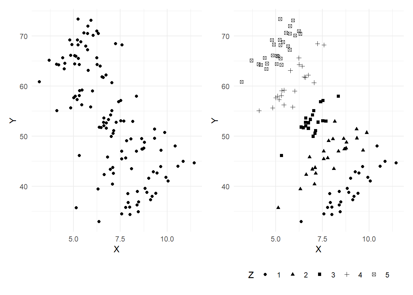
There is a clear negative relationships between \(Y\) and \(X\). However, in panel (b) we see that \(Y\) and \(X\) are in fact positively correlated when \(Z\) is fixed at some specific value. However, there is a positive relationship between \(Y\) and \(Z\), and a negative one between \(Z\) and \(X\), the net effect of which is to sweep the scatter in the northwest direction as \(Z\) increases, turning a positive correlation between \(Y\) and \(X\) for fixed values of \(Z\) to a negative one overall.
We run two regressions below. The first is a simple linear regression of \(Y\) on \(X\). The second is a multiple linear regression of \(Y\) on \(X\) and \(Z\).
mdl1 <- lm(Y~X, data=df)
coef(summary(mdl1))
Estimate Std. Error t value Pr(>|t|)
(Intercept) 82.892162 3.2234151 25.715634 3.394337e-50
X -4.237024 0.4480503 -9.456581 3.882573e-16cat("R-squared:", summary(mdl1)$r.squared,"\n\n")R-squared: 0.431125 mdl2 <- lm(Y~X+Z, data=df)
coef(summary(mdl2)) Estimate Std. Error t value Pr(>|t|)
(Intercept) 1.133354 2.0745669 0.5463086 5.858941e-01
X 3.122025 0.2048571 15.2400162 1.473978e-29
Z 10.110311 0.2369353 42.6711993 3.639969e-73cat("R-squared:", summary(mdl2)$r.squared,"\n\n")R-squared: 0.9656532 The simple linear regression shows the negative relationship between \(Y\) and \(X\) when viewed over all outcomes of \(Z\). The multiple regression disentangles the effect of \(X\) and \(Z\) on \(Y\). In this case, inclusion of \(Z\) has also reduced the standard error on the estimate of the coefficient on \(X\) despite the reduced variation in \(X\). This is because \(Z\) accounts for a very substantial proportion of the variation in \(Y\), as can be seen from the substantial increase in \(R^2\) when it is included (i.e., including \(W\) reduces the variance of the noise term by a lot).
We replicate below the multi-step approach to obtaining the coefficient estimate on \(X\):
mdl1a <- lm(Y~Z, data=df)
r_yz <- residuals(mdl1a)
mdl1b <- lm(X~Z, data=df)
r_xz <- residuals(mdl1b)
df$r_yz <- r_yz
df$r_xz <- r_xz
coef(summary(lm(r_yz~r_xz-1, data=df)))  # "-1" in the formula means exclude the intercept
Estimate Std. Error t value Pr(>|t|)
r_xz 3.122025 0.2031283 15.36972 4.896607e-30The numerical estimate of the coefficient on r_xz is identical to that on X in the previous regression. The standard errors are similar, but not the same. We emphasize that the auxiliary regression approach is for illustrative purposes only. The standard errors, t-statistic, etc. should all be taken from the previous (multiple) regression.
The plots in Fig. 6.2 illustrate the effect of ‘controlling’ for Z.
plot_theme <- theme_minimal() + theme(legend.position = "none")
p1 <- ggplot(data=df) + geom_point(aes(x=X,y=Y, shape=as.factor(Z))) +
      xlim(c(2.5,12.5)) + ylim(c(30,80)) + plot_theme
p2 <- ggplot(data=df) + geom_point(aes(x=r_xz,y=Y, shape=as.factor(Z))) +
        xlim(c(-5,5)) + ylim(c(30,80)) + plot_theme
p3 <- ggplot(data=df) + geom_point(aes(x=r_xz,y=r_yz, shape=as.factor(Z))) +
        xlim(c(-5,5)) + ylim(c(-25,25)) + plot_theme
p1|p2|p3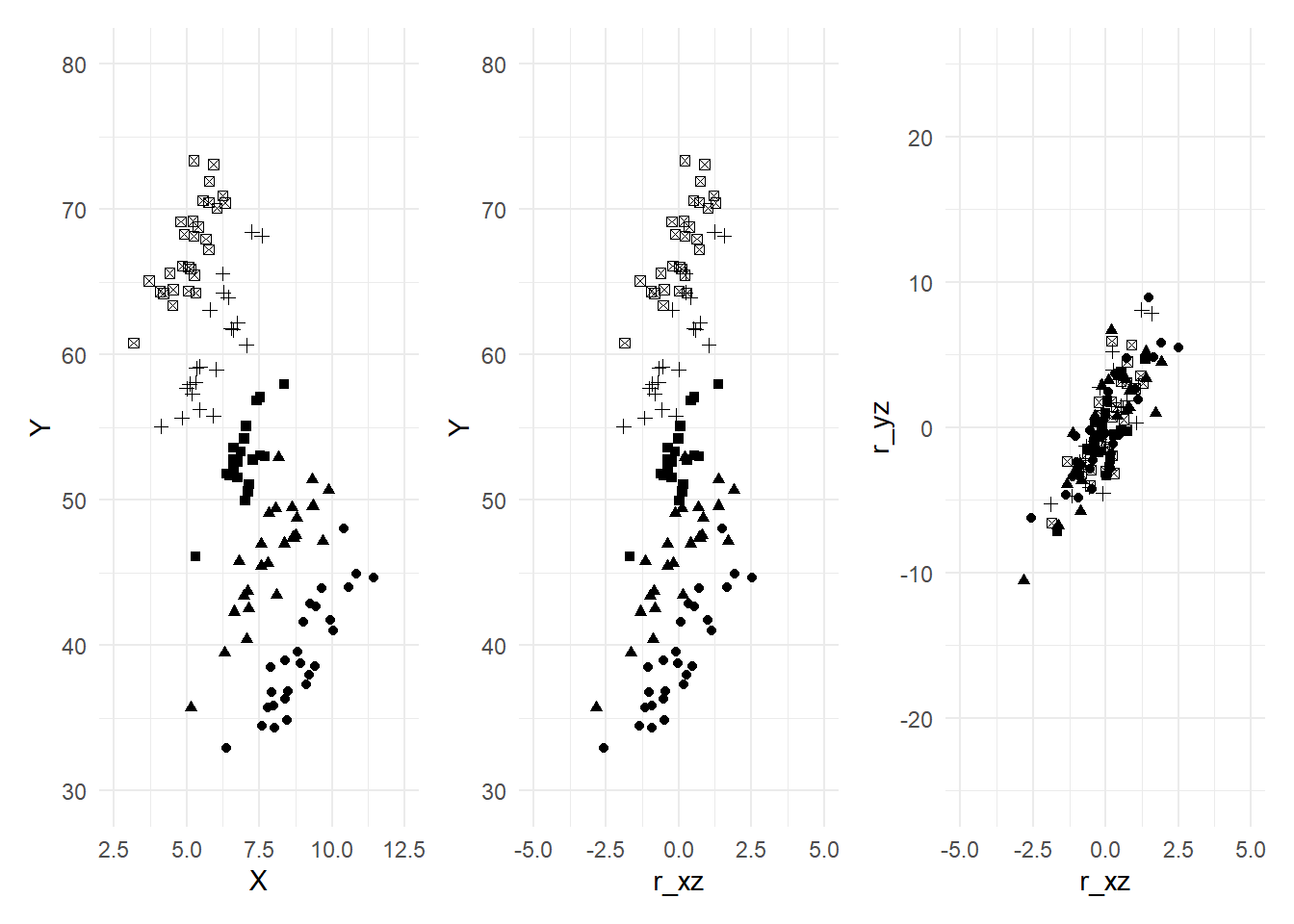
The range of the y-axis in the three plots are the same (30 to 80 in the first two, -25 to 25 in the third). Likewise the range of the x-axis is the same across all three plots (2.5 to 12.5 in the first, -5 to 5 in the second and third). This allows you to see the reduced variation in the variables. When we regress \(X\) on \(Z\) and take the residuals, we remove the effect of \(Z\) on \(X\) and also center the residuals around zero (OLS residuals always have sample mean zero). You can see from the second diagram that the variation in \(X\) is reduced, which tends to increase the estimator variance. You can also see that the negative slope has been turned into a positive one, albeit with a lot of noise. By removing the effect of \(Z\) on \(Y\) (which we do when we include \(Z\) in the regression), we reduce the variation on \(Y\). This reduces the estimator variance. The slope coefficient in the simple regression of the data in the last panel gives the effect of \(X\) on \(Y\), controlling for \(Z\).
6.4 Hypothesis Testing
To test if \(\beta_k\) is equal to some value \(r_k\) in population, we can again use the t-statistic as in the simple linear regression case: \[ t = \frac{\hat{\beta}_k - r_k}{\sqrt{\widehat{var}[\hat{\beta}_k]}}. \] If the noise terms are conditionally normally distributed, then the \(t\)-statistic has the \(t\)-distribution, with degrees-of-freedom \(N-K\) where \(K=3\) in the two-regressor case with intercept. If we do not assume normality of the noise terms, then (as long as the necessary CLTs apply) we use instead the approximate test, using the \(t\)-statistic as defined above, but using the rejection region derived from the standard normal distribution. You can also test whether a linear combination of the parameters are equal to some value. For example, in the regression \[ Y = \beta_0 + \beta_1 X + \beta_2 Z + \epsilon \] you can test, say, \(H_0: \beta_1 + \beta_2 = 1 \text{ vs } H_A: \beta_1 + \beta_2 \neq 1\). The \(t\)-statistic in this case is \[ t = \frac{\hat{\beta}_1 + \hat{\beta}_2 - 1}{\sqrt{\widehat{var}[\hat{\beta}_1+\hat{\beta}_2]}}. \] To compute this you will need the covariance of \(\hat{\beta}_1\) and \(\hat{\beta}_2\), the derivation of which we leave for a later chapter.
Example 6.6 Suppose the production technology of a firm can be characterized by the “Cobb-Douglas Production Function”: \[ Q(L,K) = AL^\alpha K^\beta \] where \(Q(L,K)\) is the quantity produced using \(L\) units of labor and \(K\) units of capital. The constants \(A\), \(\alpha\) and \(\beta\) are the parameters of the model. If we multiply the amount of labor and capital by \(c\), we get \[ Q(cL,cK) = A(cL)^\alpha (cK)^\beta = c^{\alpha+\beta}AL^\alpha K^\beta. \] The sum \(\alpha + \beta\) therefore represents the ‘returns to scale’. If \(\alpha + \beta = 1\), then there is constant returns to scale, e.g., doubling the amount of labor and capital (\(c=2\)) results in the doubling of total production. If \(\alpha + \beta > 1\) then there is increasing returns to scale, and if \(\alpha + \beta < 1\), we have decreasing returns to scale. A logarithmic transformation of the production function gives \[ \ln Q = \ln A + \alpha \ln L + \beta \ln K. \] If we have observations \(\{Q_i, L_i, K_i\}_{i=1}^N\) of the quantities produced and amount of labor and capital employed by a set of similar firms in an industry, we could estimate the production function for that industry using the regression \[ \ln Q_i = \ln A + \alpha \ln L_i + \beta \ln K_i + \epsilon_i. \] A test for constant returns to scale would be the test \[ H_0: \alpha + \beta = 1 \text{ vs } H_A: \alpha + \beta \neq 1. \]
Example 6.7 In the previous chapter, we estimated \(\ln(earnings)\) on \(height\) using data in earnings.xlsx and obtained a statistically significant effect of height on earnings. We conjectured that the regression may be measuring a ‘gender gap’ in wages rather than a ‘height gap’, with \(height\) acting as a proxy for the sex of the subjects. We now attempt to control for the sex of the subjects by including a dummy variable \(male\) which is one when an observation is of a male subject, zero otherwise.
df_earnings <- read_excel("data\\earnings.xlsx")
mdl_earnings <- lm(log(earnings) ~ height + male, data=df_earnings)
summary(mdl_earnings)
Call:
lm(formula = log(earnings) ~ height + male, data = df_earnings)

Residuals:
     Min       1Q   Median       3Q      Max
-2.17607 -0.35889 -0.01983  0.33112  2.13062

Coefficients:
            Estimate Std. Error t value Pr(>|t|)
(Intercept) 1.003213   0.539157   1.861  0.06333 .
height      0.025079   0.008332   3.010  0.00273 **
male        0.183117   0.070562   2.595  0.00971 **
---
Signif. codes:  0 '***' 0.001 '**' 0.01 '*' 0.05 '.' 0.1 ' ' 1

Residual standard error: 0.56 on 537 degrees of freedom
Multiple R-squared:  0.09794,   Adjusted R-squared:  0.09458
F-statistic: 29.15 on 2 and 537 DF,  p-value: 9.564e-13
Inclusion of the \(male\) dummy variable has reduced the size of the estimate of the \(height\) coefficient to 2.5 percent per inch in height (previously it was estimated at four percent). The estimate is still quite economically significant, and also still statistically significant. Perhaps \(height\) does have a direct effect on \(\ln(earnings)\), but it is more likely that there are yet more factors that need to be controlled for.
In some cases, we may wish to test multiple hypotheses, e.g., in the two-variable regression, we may wish to test \[ H_0: \beta_1 = 0 \; \text{ and } \; \beta_2 = 0 \; \text{ vs } \; H_A: \beta_1 \neq 0 \;\text{or}\; \beta_2 \neq 0. \] One possibility would be to do individual \(t\)-tests for each of the two hypotheses, but we should be aware that two individual 5% tests is not equivalent to a joint 5% test. The following example illustrates this problem.
Example 6.8 We generate 100 observations of three uncorrelated variables \(X\), \(Y\) and \(Z\). We regress \(Y\) on \(X\) and \(Z\), and collect the t-statistics on \(X\) and \(Z\). We repeat the experiment 1000 times (with different draws each time, of course, but the same parameters).
set.seed(3)
nreps <- 1000
tx <- tz <- rep(NA,nreps)
N <- 100
for (i in 1:nreps){
  X <- rnorm(N, mean=0, sd=2)
  Z <- rnorm(N, mean=0, sd=2)
  Y <- rnorm(N, mean=0, sd=2)
  df_test <- data.frame(X,Y,Z)
  mdlsim <- lm(Y~X+Z, data=df_test)
  tx[i] <- coef(summary(mdlsim))[2,'t value']
  tz[i] <- coef(summary(mdlsim))[3,'t value']
}
rjt_x <- sum(tx<qt(0.025,N-3) | tx>qt(0.975,N-3))/nreps
cat("Freq. of rejection of Beta_X = 0:", rjt_x, "\n")
Freq. of rejection of Beta_X = 0: 0.058 rjt_z <- sum(tz<qt(0.025,N-3) | tz>qt(0.975,N-3))/nreps
cat("Freq. of rejection of Beta_Z = 0:", rjt_z, "\n")Freq. of rejection of Beta_Z = 0: 0.054 rjt_x_or_z <- sum(tz<qt(0.025,197) | tz>qt(0.975,197) |
tx<qt(0.025,197) | tx>qt(0.975,197))/nreps
cat("Freq. of rejection of Beta_X = 0 and Beta_Z = 0 using two t-tests:", rjt_x_or_z, "\n")Freq. of rejection of Beta_X = 0 and Beta_Z = 0 using two t-tests: 0.112 When using a 5% t-test, we reject the (true) hypothesis that \(\beta_x = 0\) in about 6% of the experiments, close to 5%. These rejections are regardless of whether the t-test for \(\beta_z=0\) rejects or does not reject. Likewise, the 5% t-test for \(\beta_z = 0\) rejects the hypothesis 5.5% of the time, roughly five percent. However, if we say we reject \(\beta_x = 0\) and \(\beta_z = 0\) if either t-tests rejects the corresponding hypothesis, then the frequency of rejection is much larger, roughly double.
We plot the t-stats below, indicating the critical values for the individual tests. The proportion of points above the upper horizontal line or below the lower one is about 0.05. Similarly, the proportion of points to the left of the left vertical line or to the right of the right one is roughly 0.05. The number of point that meet either of the two sets of criteria is much larger, roughly the sum of the two proportions.
df_t <- data.frame(tx,tz)
ggplot(data=df_t) + geom_point(aes(x=tx,y=tz)) +
  geom_hline(yintercept = qt(0.025,N-3), lty='dashed', col='blue') +
  geom_hline(yintercept = qt(0.975,N-3), lty='dashed', col='blue') +
  geom_vline(xintercept = qt(0.025,N-3), lty='dashed', col='blue') +
  geom_vline(xintercept = qt(0.975,N-3), lty='dashed', col='blue') +
  theme_minimal()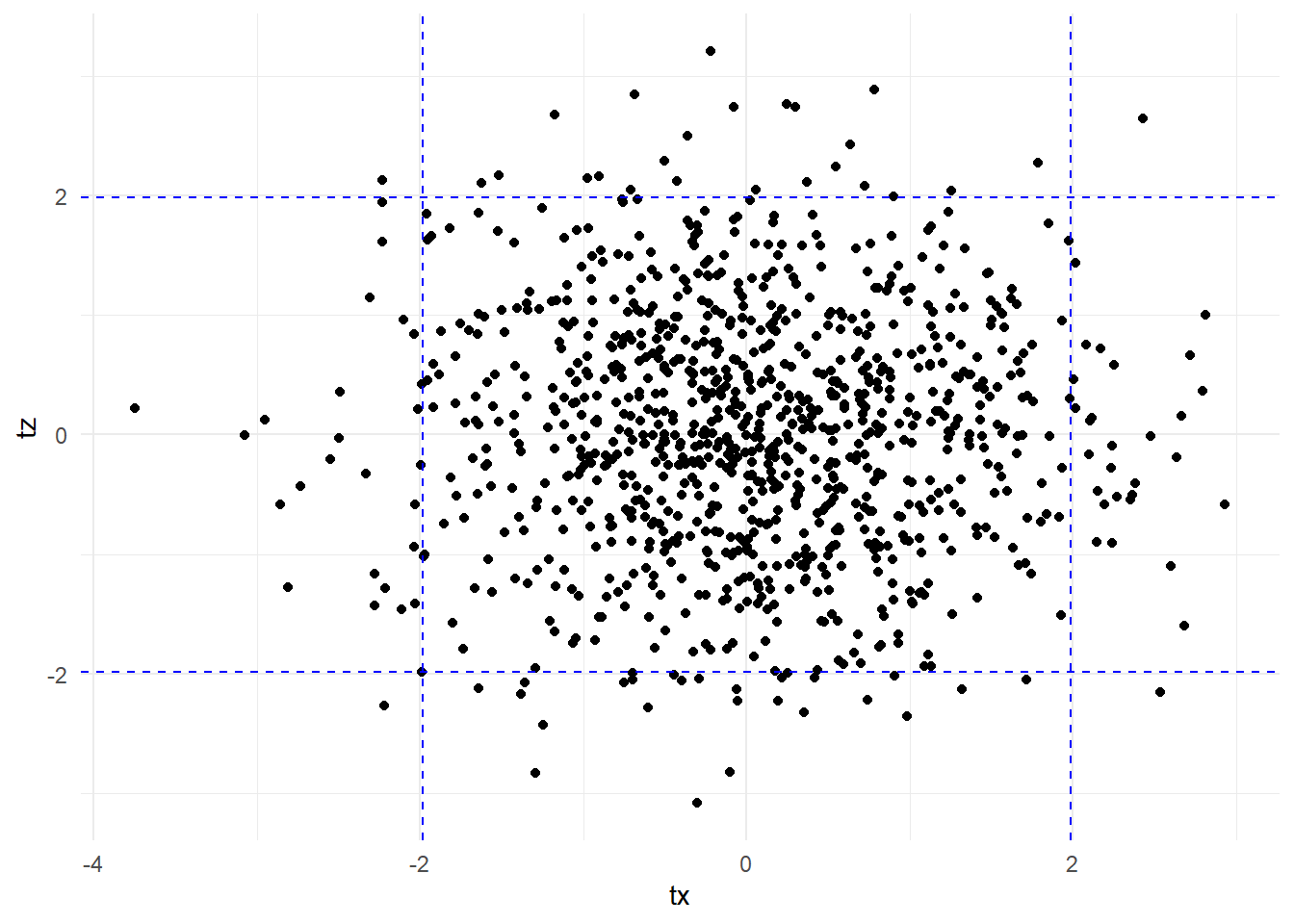
To jointly test multiple hypotheses, we can use the \(F\)-test. Suppose in the regression \[ Y = \beta_0 + \beta_1X + \beta_2 Z + \epsilon \] we wish to jointly test the hypotheses \[ H_0: \beta_1 = 1 \; \text{ and } \; \beta_2 = 0 \; \text{ vs } \; H_A: \beta_1 \neq 1 \;\text{or}\; \beta_2 \neq 0 \;\text{ (or both)}\,. \] Suppose we run the regression twice, once unrestricted, and another time with the restrictions in \(H_0\) imposed. The regression with the restrictions imposed is \[ Y = \beta_0 + X + \epsilon \] so the restricted OLS estimator for \(\beta_0\) is the sample mean of \(Y_i - X_i\), i.e., \[ \hat{\beta}_{0,r} = (1/N)\sum_{i=1}^N(Y_i - X_i). \] Calculate the \(SSR\) from both equations. The “unrestricted \(SSR\)” is \[ SSR_{ur} = \sum_{i=1}^N \hat{\epsilon}_i^2 \] where \(\hat{\epsilon}_i = Y_i - \hat{\beta}_0 - \hat{\beta}_1X_i - \hat{\beta}_2 Z_i\). The restricted \(SSR\) is \[ SSR_{r} = \sum_{i=1}^N \hat{\epsilon}_{i,r}^2 \] where \(\hat{\epsilon}_{i,r} = Y_i - \hat{\beta}_{0,r} - X_i\). Since OLS minimizes \(SSR\), imposing restrictions will generally increase the \(SSR\), and never decrease it, i.e., \[ SSR_r \geq SSR_{ur} \,. \] It can be shown that if the hypotheses in \(H_0\) are true (and the noise terms are normally distributed), then \[ F = \frac{(SSR_r - SSR_{ur})/J}{SSR_{ur}/(N-K)} \sim F_{(J,N-K)} \tag{6.22}\] where \(J\) is the number of restrictions being tested (in our example, \(J=2\)) and \(K\) is the number of coefficients to be estimated (including intercept; in our example, \(K=3\)). The F-statistic is always non-negative. The idea is that if the hypotheses in \(H_0\) are true, then imposing the restrictions on the regression would not increase the \(SSR\) by much, and \(F\) will be close to zero. On the other hand, if one or more of the hypotheses in \(H_0\) are false, then imposing them into the regression will cause the \(SSR\) to increase substantially, and the \(F\) statistic will be large. We take a very large \(F\)-statistic, meaning \[ F > F_{\alpha,J,N-K}\,, \] as statistical evidence that one or more of the hypothesis is false, where \(F_{\alpha,J,N-K}\) is the \((1-\alpha)\)-percentile of the \(F_{J,N-K}\) distribution and where \(\alpha\) is typically 0.10, 0.05 or 0.01,
Since \(R^2 = 1 - SSR/SST\), we can write the \(F\)-statistic in terms of \(R^2\) instead of \(SSR\). You are asked in an exercise to show that the \(F\)-statistic can be written as \[ F = \frac{(R_{ur}^2 -R_r^2)/J}{(1-R_{ur}^2)/(N-K)}. \] Imposing restrictions cannot increase \(R^2\), and in general will decrease it. The \(F\)-test essentially tests if the \(R^2\) drops significantly when the restrictions are imposed. If the hypotheses being tested are true, then the drop should be slight. If one or more are false, the drop should be substantial, resulting in a large \(F\)-statistic.
If you cannot assume that the noise terms are conditionally normally distributed, then you will have to use an asymptotic approximation. It can be shown that \[ JF \rightarrow_d \chi_{(J)}^2 \] as \(N \rightarrow \infty\), where \(J\) is the number of hypotheses being jointly tested, and \(F\) is the \(F\)-statistic Eq. 6.22. We refer to this as the “Chi-square Test”.
Example 6.9 We continue with Example Example 6.5. We estimate the model using lm() and store the results in mdl. We use the summary() function to display the results.
df <- read_csv("data\\multireg_eg.csv",col_types = c("n","n","n"))
mdl <- lm(Y~X+Z, data=df)
summary(mdl)
Call:
lm(formula = Y ~ X + Z, data = df)

Residuals:
   Min     1Q Median     3Q    Max
-4.369 -1.396 -0.077  1.246  6.068

Coefficients:
            Estimate Std. Error t value Pr(>|t|)
(Intercept)   1.1334     2.0746   0.546    0.586
X             3.1220     0.2049  15.240   <2e-16 ***
Z            10.1103     0.2369  42.671   <2e-16 ***
---
Signif. codes:  0 '***' 0.001 '**' 0.01 '*' 0.05 '.' 0.1 ' ' 1

Residual standard error: 2.07 on 117 degrees of freedom
Multiple R-squared:  0.9657,    Adjusted R-squared:  0.9651
F-statistic:  1645 on 2 and 117 DF,  p-value: < 2.2e-16
The t-statistics are for testing (separately) \(\beta_x=0\) and \(\beta_z=0\). The F-statistic that is reported is for testing both of these hypotheses jointly, i.e., \(H_0:\beta_x=0 \; \text{ and } \; \beta_z=0\) versus the alternative that one or both do not hold, and the p-value listed next to the F-statistic is the probability that an \(F_{(2,117)}\) random variable exceeds the computed F-statistic. In this example, we resounding reject the null that both coefficients are zero. The residual standard error is the square root of \(\widehat{\sigma^2}\), the multiple R-squared is the \(R^2\) discussed earlier. The “Adjusted R-Squared” is the modified \(R^2\) as previously discussed.
As an illustration of the general F test, suppose instead we wish to test that \(\beta_0=1\) and \(\beta_z=3\beta_x\). The restricted regression is \[ Y = 1 + \beta_x X + 3\beta_x Z + \epsilon = 1 + \beta_x (X+3Z) + \epsilon\,. \] The OLS estimator for the only parameter in the restricted regression, \(\beta_x\), can be obtained from a regression of \(Y_i - 1\) on \((X_i+3Z_i)\) with no intercept term. We have
mdlr <- lm((Y-1)~I(X+3*Z)-1, data=df)
coef(mdlr)
I(X + 3 * Z)
3.276943 The restricted residuals can be computed as \[ \hat{\epsilon}_{i,r} = Y_i - 1 - \hat{\beta}_{x,r}(X_i + 3Z_i) \] The F-statistic and associate p-value is
ehat_r  <- df$Y - 1 - coef(mdlr)[1] * (df$X + 3*df$Z)
SSR_r   <- sum(ehat_r^2)
ehat_ur <- residuals(mdl)
SSR_ur <- sum(ehat_ur^2)
df1 <- 2
df2 <- nobs(mdl) -length(coef(mdl))
F <- ((SSR_r-SSR_ur)/2)/(SSR_ur/(nobs(mdl)-length(coef(mdl))))
Fpval <- 1-pf(F, df1, df2)
X2 <- df1*F
X2pval <- 1-pchisq(X2, df1)
cat("Unrestricted SSR:", round(SSR_ur,6), "\n")
cat("Restricted SSR:", round(SSR_r,6), "\n")
cat("F-stat:",round(F,6))
cat("     p-val:",round(Fpval,6), "\n")
cat("Chi-sq:",round(X2,6))
cat("    p-val:",round(X2pval,6), "\n")
Unrestricted SSR: 501.2613
Restricted SSR: 553.7018
F-stat: 6.12009 p-val: 0.002966
Chi-sq: 12.24018 p-val: 0.002198 The function linearHypothesis() in the car package can also be used to carry out the F- and Chi-sq tests.
linearHypothesis(mdl,c('(Intercept)=1','Z-3*X = 0'), test="F")Linear hypothesis test
Hypothesis:
(Intercept) = 1
- 3 X + Z = 0
Model 1: restricted model
Model 2: Y ~ X + Z
Res.Df RSS Df Sum of Sq F Pr(>F)
1 119 553.70
2 117 501.26 2 52.44 6.1201 0.002966 **
---
Signif. codes: 0 '***' 0.001 '**' 0.01 '*' 0.05 '.' 0.1 ' ' 1linearHypothesis(mdl,c('(Intercept)=1','Z-3*X = 0'), test="Chisq")Linear hypothesis test
Hypothesis:
(Intercept) = 1
- 3 X + Z = 0
Model 1: restricted model
Model 2: Y ~ X + Z
Res.Df RSS Df Sum of Sq Chisq Pr(>Chisq)
1 119 553.70
2 117 501.26 2 52.44 12.24 0.002198 **
---
Signif. codes: 0 '***' 0.001 '**' 0.01 '*' 0.05 '.' 0.1 ' ' 16.5 Exercises
Exercise 6.1 Each of the following regressions produces a sample regression function whose slope is \(\hat{\beta}_1\) when \(X_i < \xi\) and \(\hat{\beta}_1 + \hat{\alpha}_1\) when \(X_i \geq \xi\). Which of them produces a sample regression function that is continuous at \(\xi\)?
\(Y_i = \beta_0 + \beta_1 X_i + \alpha_1 D_i X_i + \epsilon\) where \(D_i\) is a dummy variable with \(D_i = 1\) if \(X_i > \xi\), \(D_i = 0\) otherwise;
\(Y_i = \beta_0 + \alpha_0D_i + \beta_1 X_i + \alpha_1 D X_i + \epsilon\);
\(Y_i = \beta_0 + \beta_1 X_i + \alpha_1 (X_i-\xi)_+ + \epsilon_i\)where \[ (X_i-\xi)_+ = \begin{cases} X_i - \xi & \text{if} \; X_i > \xi \;, \\ 0 & \text{if} \; X_i \leq \xi\;. \end{cases} \]
Exercise 6.2 The following is a “piecewise quadratic regression” model \[ Y = \beta_0 + \beta_1X + \beta_2X^2 + \beta_3(X-\xi)_+^2 + \epsilon\,,\,E[\epsilon | X] = 0. \] where \[ (X_i-\xi)_+^2 = \begin{cases} (X_i - \xi)^2 & \text{if} \; X_i > \xi \;, \\ 0 & \text{if} \; X_i \leq \xi\;. \end{cases} \] Show that the PRF \(E[Y|X]\) is “piecewise quadratic”, following one quadratic equation when \(X\leq\xi\), and another when \(x > \xi\). Show that the PRF is continuous, with continuous first derivative.
Exercise 6.3 Suppose your estimated sample regression function is \[ \widehat{wage} = -68.28 + 4.163\,age - 0.052\,age^2 \] where \(\hat{\alpha}_0\) and \(\hat{\alpha}_1\) are positive and \(\hat{\alpha}_2\) is negative. At what age are wages predicted to start declining with age? Does the intercept have any reasonable economic interpretation?
Exercise 6.4 Prove Eq. 6.14.
Exercise 6.5 Show that the \(F\)-statistic in Eq. 6.22 can be written as \[ F = \frac{(R_{ur}^2 - R_r^2)/J}{(1-R_{ur}^2)/(N-K)} \] where \(R_{ur}\) and \(R_r\) are the \(R^2\) from the unrestricted and restricted regressions respectively, \(J\) is the number of restrictions being tested, \(N\) is the number of observations used in the regression, and \(K\) is the number of coefficient parameters in the unrestricted regression model (including intercept). What does this expression simplify to when testing that all the slope coefficients (excluding the intercept) are equal to zero?
Exercise 6.6 Modify the code in Example 6.8 to collect the F-statistic for jointly testing \(\beta_x = 0\) and \(\beta_z=0\). Show that the 5% F-test is empirically correctly sized, meaning that the frequency of rejection in the simulation is in fact around 5%.
Exercise 6.7 Suppose \[ \begin{aligned} Y &= \alpha_0 + \alpha_1 X + \alpha_2 Z + u \\ Z &= \delta_1 X + v \end{aligned} \] where \(u\) and \(v\) are independent zero-mean noise terms. Suppose you have a random sample \(\{Y_i,X_i,Z_i\}_{i=1}^N\) and you ran the regression \[ Y_i = \beta_0 + \beta_1 X_i + \epsilon_i. \] Show that the OLS estimator \(\hat{\beta}_1\) will be biased for \(\alpha_1\). What is its expectation? Show that the prediction rule \[ \hat{Y}=\hat{\beta}_0 + \hat{\beta}_1X \] still provides unbiased predictions, but that the prediction error variance is greater than the prediction error variance from using the prediction rule \[ Y = \hat{\alpha}_0 + \hat{\alpha}_1 X + \hat{\alpha}_2 Z \] where \(\hat{\alpha}_0\), \(\hat{\alpha}_1\), and \(\hat{\alpha}_2\) are the OLS estimators for \(\alpha_0\), \(\alpha_1\) and \(\alpha_2\) in the regression \[ Y_i = \alpha_0 + \alpha_1 X_i + \alpha_2 Z_i + u_i \]
Exercise 6.8 Verify all of the results reported in Example 6.9 by calculating them directly using the formulas developed in the notes (in particular, verify the coefficient estimates, standard errors, t-statistics and associated p-values, the residual standard error, the multiple R-squared and Adjusted R-squared, the F-statistic and the corresponding p-value).
If we use \(X_{1}\), \(X_{2}\), etc. to denote different variables, then the \(i\)th observation of regressor \(X_{j}\) will be denoted \(X_{j,i}\). If we use \(X\), \(Y\), \(Z\), to denote different variables, then the \(i\)th observation of these variables will be denoted \(X_{i}\), \(Y_{i}\), \(Z_{i}\).↩︎