library(tidyverse)   # For data handling and visualization
library(patchwork)   # ]
library(gridExtra)   # ] For plot management
library(latex2exp) # ]5 Simple Linear Regression
Simple linear regression is a framework for developing empirical models of the form \[ \hat{Y} = \hat{\beta}_0 + \hat{\beta}_1 X \tag{5.1}\] for the purpose of prediction, inferring causality from \(X\) to \(Y\), testing hypotheses regarding \(X\) and \(Y\), among other applications. This chapter describes and studies this framework. The simple linear regression framework will in many instances turn out to be insufficient for predictive, causal inference and testing applications, but it is a good place to start, both as a first step towards mastering the principles and technicalities of more advanced frameworks, and as a way to better understand the issues involved in these applications.
We focus on cross-sectional regressions in this chapter. Time series regressions are discussed in a later chapter. Our initial discussions will also focus on the problem of prediction, although we will also discuss hypothesis testing and issues involved in trying to interpret regression results as causal effects.
The R code in this chapter uses the following packages.
5.1 The Simple Linear Regression Framework
Suppose you have observations \(\{X_{i}, Y_{i}\}_{i=1}^{N}\) and you want to build an empirical model of the form Eq. 5.1 for predicting \(Y\) for new observations at given values of \(X\). For example, you want to predict the price \(Y\) of new houses to be built \(X=x\) distance from town center, or for predicting how much new customers with income levels \(X=x\) are likely to spend on some product. We’ll keep \(X\) and \(Y\) generic for the moment.
You know that the point prediction that minimize mean squared prediction error is the conditional mean (and suppose that minimizing mean squared prediction error is your objective). You plan to use the empirical model Eq. 5.1 as an estimate of the conditional expectation \[ E[Y|X] \approx \widehat{E}[Y|X] = \hat{\beta}_0 + \hat{\beta}_1 X\,. \] New observations with \(X = x\) will be predicted to have \(\hat{Y} = \hat{\beta}_{0} + \hat{\beta}_{1}x\). Estimating Eq. 5.1 amounts to using your data to come up with appropriate values of \(\hat{\beta}_{0}\) and \(\hat{\beta}_{1}\). What method should you use? If you choose to use ordinary least squares (OLS) as described in Section 2.4, under what conditions would that give you “good” estimates of the conditional expectation? Are you able to give some indication of how much your predictions can be trusted? Is the supposed linear form of the conditional expectation appropriate in the first place?
We answer these questions by first laying out a set of assumptions, and showing that OLS works well in under these assumptions. Then we ask what happens when one or more of the assumptions fail. Later chapters will discuss how the basic framework can be modified to such situations. In practice, diagnostic assessments are made to ascertain if the assumptions in the basic framework are appropriate for your particular application. These will usually include both data-based approaches (are the assumptions consistent with the data?) and as well as assessments based on a knowledge of economics. Assumptions and estimation methods are then modified accordingly.
Let \(X\) and \(Y\) be your variables of interest, and let \(\{X_i,Y_i\}_{i=1}^N\) be your data sample. We suppose for the moment that you have a cross-sectional sample, i.e., you have data on a sample of individuals (this could be individual people, individual firms, …) that can be considered to have been collected at a single point in time. We consider other data structures in later chapters.
Assumption Set A: Suppose that (A1) there are two values \(\beta_0\) and \(\beta_1\) such that the random variable \(\epsilon\), defined as \[ \epsilon = Y - \beta_{0} - \beta_{1} X, \] satisfies
(A2) \(E[\epsilon|X] = 0\),
(A3) \(var[\epsilon|X] = \sigma^2\).
Suppose also that
(A4) \(\{X_i,Y_i\}_{i=1}^N\) is a random sample from the population of interest, and
(A5) \(\sum_{i=1}^N (X_i-\overline{X})^2 > 0\).
It is important to understand that we are placing ourselves in a position prior to observing data, and treating the \(X_{i}\) and \(Y_{i}\) in the sample as random variables. We want to know if the methods to be proposed for building the empirical model will work in general situations conforming to the scenario described in Assumption Set A.
Assumption A2 implies that
\[
E[Y|X] = \beta_0 + \beta_1 X
\tag{5.2}\]
We call Eq. 5.2 the Population Regression Function (PRF). For obvious reasons, we call \(\beta_{0}\) the “intercept”, and \(\beta_{1}\) the “slope coefficient”. The variable \(\epsilon\) is called the “error” or “noise” term. The variable \(Y\) is the “dependent/explained/response/predicted variable”, or “regressand”. The variable \(X\) is the “independent/explanatory/control variable” or “regressor”. In predictive applications, it is often called the “predictor”. Assumption A2 also implies that \[ \mathrm{cov}[X,\epsilon]=0\,, \] and \[ \beta_{0} = E[Y] - \beta_{1}E[X] \quad \text{and} \quad \beta_{1} = \frac{\mathrm{cov}[X,Y]}{var[X]}\,. \]
Assumption A3 is called “conditional homoskedasticity”. It says that the variance of the noise term does not depend on \(X\). If A3 holds, we should expect that the spread of the sample realizations about the regression line should be more or less even, so that, roughly speaking, each observation is equally informative about the regression line. If A3 does not hold, we say that there is “conditional heteroskedasticity” in the noise term.1 Incidentally, if A2 holds, then we can write A3 as \(E[\epsilon^{2}|X] = \sigma^{2}\).
Example 5.1 The file heterosk.csv contains observations on three variables \(X\), \(Y\) and \(Z\). We plot observations of \(Y\) against \(X\) in panel (a), and \(Z\) against \(X\) in panel (b) using data in heterosk.csv. Visually, assumption A3 appears appropriate if your data behaves as in (a) in Fig. 5.1, but almost surely does not hold if your data behaves as in (b). In the latter case, there is strong visual evidence that the variance of \(\epsilon\) increases with \(X\).
df_het <- read_csv("data\\heterosk.csv",col_types = c("n","n","n"))
plt_het1a <- ggplot(data=df_het) + geom_point(aes(x=x,y=z), size=1) +
      ggtitle("(a)") + theme_classic()
plt_het1b <- ggplot(data=df_het) + geom_point(aes(x=x,y=y), size=1) +
      ggtitle("(b)") + theme_classic()
plt_het1a | plt_het1b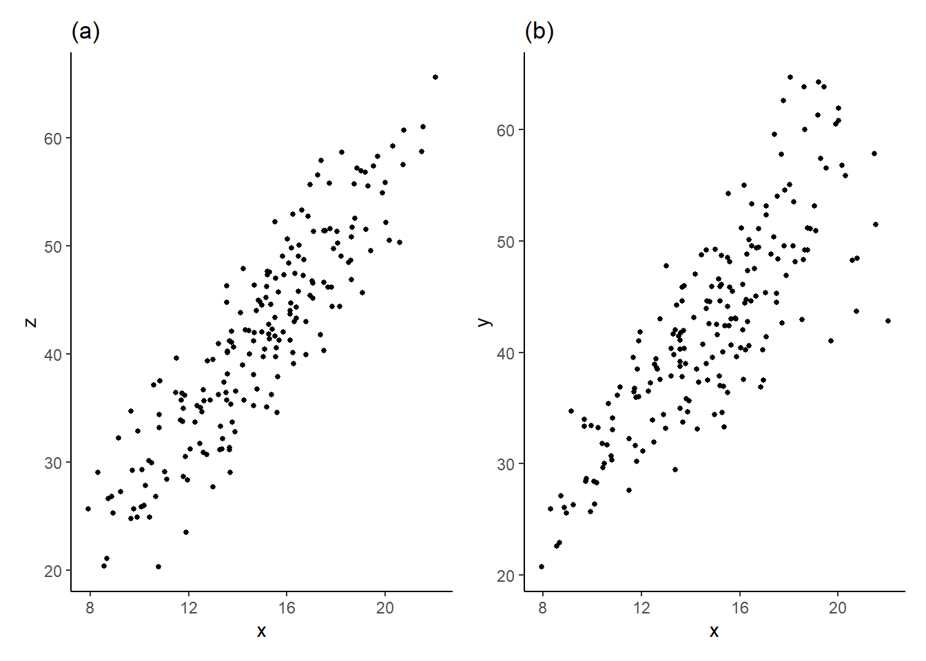
One application where the data may appear as in (b) is when \(Y\) is expenditure and \(X\) is income. Low income earners may have to spend most of their earnings on necessary purchases, with little room for variation, whereas high income earners have considerably more discretion in how much of their income to spend or save.
There is a lot packed into the phrase “random sample from the population of interest”. “Random sample” is usually taken to mean that the sample \(\{X_i,Y_i\}_{i=1}^N\) are independently and identically distributed draws. From a data sampling perspective, the term means that you have a representative draw from the population of interest, without favoring draws from segments of the population with with certain characteristics. Suppose you are measuring the distribution of heights in an adult population of a certain country. If your sampling process somehow makes it more likely to sample males than females. The result will be that the distribution of heights in your sample will not be representative of your population. You want each member of the population to have an equal chance of getting sampled, so that your sample has the same mix of characteristics as the entire population. If your sample comprises whole families, then there will be dependence in heights within members of the same family. In the latter case, you could still get a representative sample of the population, but you would need a much larger sample, and calculations of statistics like variances will need to take the dependence into consideration.
We will discuss each of these assumptions in greater detail shortly, when they might fail to hold, and the consequences. For now, we consider OLS estimation of the population regression function, and the properties of the estimators under Assumption Set A.
5.2 Ordinary Least Squares
Under Assumption A2, we can write \[ Y_{i} = \beta_{0} + \beta_{1} X_{i} + \epsilon_{i}\;,\;\;i = 1,2,...,N. \] For any estimators \(\hat{\beta}_0\) and \(\hat{\beta}_1\) (whether obtained by OLS or otherwise), define the fitted values to be \[ \hat{Y_i} = \hat{\beta}_0 + \hat{\beta}_1X_i , i=1,2,...,N \tag{5.3}\] and the residuals to be \[ \hat{\epsilon}_i = Y_i - \hat{Y_i} = Y_i - \hat{\beta}_0 - \hat{\beta}_1X_i , i=1,2,...,N. \tag{5.4}\] Ordinary Least Squares (OLS) chooses \(\hat{\beta}_{0}^{ols}\) and \(\hat{\beta}_{1}^{ols}\) to minimize the sum of squared residuals (SSR): \[ \text{OLS: Choose } \hat{\beta}_0, \hat{\beta}_1 \text{ to minimize } SSR = \sum_{i=1}^N \hat{\epsilon_i}^2 = \sum_{i=1}^N (Y_i - \hat{\beta}_0 - \hat{\beta}_1X_i)^2. \tag{5.5}\] We have already seen in Section 2.4 how the minimization problem (5.5) can be solved. The first order conditions are: \[ \begin{aligned} \left.\frac{\partial SSR}{\partial \hat{\beta}_0}\right| _{\hat{\beta}_0^{ols},\,\hat{\beta}_1^{ols}} &= -2\sum_{i=1}^N(Y_i-\hat{\beta}_0^{ols}-\hat{\beta}_1^{ols}X_i) = 0 \\ \left.\frac{\partial SSR}{\partial \hat{\beta}_1}\right| _{\hat{\beta}_0^{ols},\,\hat{\beta}_1^{ols}} &= -2\sum_{i=1}^N(Y_i-\hat{\beta}_0^{ols}-\hat{\beta}_1^{ols}X_i)X_i=0 \end{aligned} \tag{5.6}\] where we use the notation \(\left.\frac{\partial SSR}{\partial \hat{\beta}_0}\right|_{\hat{\beta}_0^{ols},\,\hat{\beta}_1^{ols}}\) to refer to the derivative \(\frac{\partial SSR}{\partial \hat{\beta}_0}\) evaluated at \(\hat{\beta}_0^{ols}\) and \(\hat{\beta}_1^{ols}\), and likewise for \(\left.\frac{\partial SSR}{\partial \hat{\beta}_1}\right|_{\hat{\beta}_0^{ols},\,\hat{\beta}_1^{ols}}\). Solving the first order conditions in Eq. 5.6 gives \[ \begin{aligned} \hat{\beta}_0^{ols} &= \overline{Y} - \hat{\beta}_1^{ols}\overline{X} \\ \hat{\beta}_1^{ols} &= \frac{\sum_{i=1}^N (Y_i-\overline{Y})X_i}{\sum_{i=1}^N(X_i-\overline{X})X_i} = \frac{\sum_{i=1}^N (X_{i} - \overline{X})(Y_i-\overline{Y})}{\sum_{i=1}^N(X_i-\overline{X})^{2}}\,. \end{aligned} \tag{5.7}\] You showed in an exercise that the second-order condition for a strict global minimum holds, so that \(\hat{\beta}_0^{ols}\) and \(\hat{\beta}_1^{ols}\) do in fact solve the minimization problem (5.5). The OLS fitted values and OLS residuals are \[ \begin{aligned} \hat{Y}_i^{ols} \;&=\; \hat{\beta}_0^{ols} + \hat{\beta}_1^{ols} X_i \\ \hat{\epsilon}_i^{ols} \;&=\; Y_i - \hat{Y}_i^{ols} \;=\; Y_i - \hat{\beta}_0^{ols} - \hat{\beta}_1^{ols}X_i \end{aligned} \] for \(i=1,2,\dots,N\). The OLS Sample Regression Function (SRF) is the line \[ \hat{Y}^{ols} = \hat{\beta}_0^{ols} + \hat{\beta}_1^{ols} X\,. \] In all that follows, we will drop the “OLS” superscript from the estimators, fitted values and residuals. These are assumed to be OLS estimators, fitted values and residuals. Where we need to discuss non-OLS estimators, we will indicate those estimators in some way.
We have seen that several algebraic identities hold under OLS estimation. We summarize them briefly below.
The first-order conditions can also be written as \[ \begin{gathered} \sum_{i=1}^N \hat{\epsilon}_{i} = 0 \\ \sum_{i=1}^N X_{i} \hat{\epsilon}_{i} = 0 \end{gathered} \tag{5.8}\] It follows that OLS residuals have zero sample mean and zero sample covariance with the regressors: \[ \begin{gathered} \frac{1}{N}\sum_{i=1}^N \hat{\epsilon}_{i} = 0 \\ \text{sample cov}[\hat{\epsilon}_{i}, X_{i}] = \frac{1}{N}\sum_{i=1}^N (\hat{\epsilon}_{i}-\overline{\hat{\epsilon}})(X_{i}-\overline{X}) = \frac{1}{N} \sum_{i=1}^{N} X_{i} \hat{\epsilon}_{i} = 0\,. \end{gathered} \] We describe the condition \(\sum_{i=1}^{N} X_{i} \hat{\epsilon}_{i} = 0\) by saying that the OLS residuals \(\hat{\epsilon}_{i}\) and the regressors \(X_{i}\) are orthogonal.
The fitted values and the residuals are also orthogonal: \[ \sum_{i=1}^N \hat{Y}_i \hat{\epsilon}_{i} = \hat{\beta}_0\sum_{i=1}^N \hat{\epsilon}_{i} + \hat{\beta}_1\sum_{i=1}^N \hat{X_{i}\epsilon}_{i} = 0\,. \]
The regressand and fitted values always have the same sample average \[ \overline{Y} = \overline{\hat{Y}}\,, \qquad \text{where}\;\; \overline{\hat{Y}} = (1/N) \sum_{i=1}^{N} \hat{Y}_{i} \] and the sample regression line (the fitted line) passes through the point \((\overline{X}, \overline{Y})\), i.e., \[ \overline{Y} = \hat{\beta}_{0} + \hat{\beta}_{1} \overline{X}\,. \]
We have the variance decomposition \[ \sum_{i=1}^N (Y_i - \overline{Y})^2 = \sum_{i=1}^N (\hat{Y}_i - \overline{\hat{Y}})^2 + \sum_{i=1}^N \hat{\epsilon}_i^2\,, \tag{5.9}\] which is often read as “Sum of Squared Total = Sum of Squared Explained + Sum of Squared Residuals” or “SST = SSE + SSR”. From this decomposition, we define the Goodness-of-Fit measure \[ R^2 = 1 - \frac{SSR}{SST}\;. \tag{5.10}\] The \(R^2\) has the interpretation as the proportion of variation in \(Y_i\) that is accounted2 for by \(\hat{Y}_i\), or by \(X_{i}\), since \(\hat{Y}_{i}\) is just a linear function of \(X_{i}\).
Many of these properties require that the intercept term be included in the regression.
Example 5.2 Suppose the PRF is \[ E[Y|X] = 2 + 1.5X \] This is plotted as a blue dashed line on the left panel in Fig. 5.2. You do not observe this line. All you observe are the data points shown as black dots.
# Simulated Data
set.seed(888)                             # For replicability
X <- rnorm(10, mean=5, sd=2)              # Simulating some data
Y <- 2 + 1.5*X + rnorm(10, mean=0, sd=3)
df <- data.frame(X, Y)
# Fit OLS and get predicted values
Ybar <- mean(df$Y); Xbar <- mean(df$X)
b1hat <- cov(df$X, df$Y)/var(df$X)
b0hat <- Ybar - b1hat*Xbar
df <- df %>%
  mutate(Yhat = b0hat + b1hat*X,  # add fitted values to df data frame
         ehat = Y - Yhat) %>%
  arrange(X)
# Plot data and lines
p1 <- df %>%  ggplot(aes(x=X,y=Y)) +
  geom_point(size=1.5) + geom_line(aes(x=X, y=Yhat), size=0.6) +
  theme_minimal() + ylab(TeX('Y, $\\hat{Y}$')) + theme(aspect.ratio = 0.8) +
  geom_abline(intercept=2, slope=1.5, col='blue', lty='dashed', lwd=0.6) +
  geom_segment(x=df$X, xend=df$X, y=df$Y, yend=df$Yhat, lty='dotted') +
  annotate(geom="text", x=4.5, y=11.5,
           label=TeX("$E\\[Y|X\\]=\\beta_0 + \\beta_1X_1$"), col="blue")
p1 + gridExtra::tableGrob(round(df[,c("X","Y")],4), theme=ttheme_minimal()) +
  plot_layout(widths=c(2.5,1))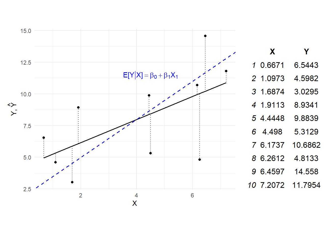
The sample regression function is shown in black, obtained by ordinary least squares. The vertical distances from the data points to the estimated line are shown as dashed line. OLS chooses the black line to minimize the sum of squared lengths of these dotted lines. The parameter estimates are
print(c("b0hat" = b0hat, "b1hat" = b1hat)) b0hat b1hat
4.3473024 0.9078149 The residuals have zero sample mean and are uncorrelated with the regressors:
## results will be up to computer precision
cat("sample mean of residuals: ", mean(df$ehat), "\n")
cat("sample covariance, residuals and regressor: ", cov(df$ehat, df$X), "\n")
sample mean of residuals: 0
sample covariance, residuals and regressor: 2.607868e-16 If you plot the point \((\overline{X}, \overline{Y})\) in the figure, you will find that it lies on the estimated line (we did not do this in the figure). The \(R^2\) for this regression is
SSR <- sum(df$ehat^2)  # we defined SSR
SST <- sum((df$Y-mean(df$Y))^2)
Rsqr <- 1 - SSR/SST
Rsqr
[1] 0.3687383In Example 5.2, the estimated regression line does not coincide with the true population regression line. Of course, this will be the case in general, since the sample regression line is only an estimate of the population regression line. The question is how the OLS procedure described here will perform on average in situations where the circumstances described in Assumption Set A hold. In the next section, we argue that, from a certain perspective, you cannot do much better than OLS.
5.2.1 Statistical Properties of OLS Estimators
It turns out that OLS produces unbiased and efficient estimators of \(\beta_{0}\) and \(\beta_{1}\), and therefore of \(E[Y|X]\), under Assumption Set A. In the arguments below we focus on \(\beta_{1}\); similar arguments hold for \(\beta_{0}\). We first note that \(\hat{\beta}_1\) can be written as \[ \begin{aligned} \hat{\beta}_1 &= \frac{\sum_{i=1}^{N} (X_{i} - \overline{X})Y_{i}}{\sum_{i=1}^{N} (X_{i} - \overline{X})^{2}} \\ &= \sum_{i=1}^N w_iY_i \;\; \text{ where } \;w_{i} = \dfrac{(X_i-\overline{X})}{\sum_{i=1}^N(X_i-\overline{X})^2}\\ &= \sum_{i=1}^N w_i(\beta_0 + \beta_1X_i + \epsilon_i) \\ &= \beta_0\sum_{i=1}^N w_i + \beta_1\sum_{i=1}^N w_iX_i + \sum_{i=1}^N w_i\epsilon_i \\ &= \beta_1 + \sum_{i=1}^N w_i\epsilon_i\,. \end{aligned} \tag{5.11}\] The second line says that \(\hat{\beta}_{1}\) is a “linear estimator”. The last line uses the fact that \[ \begin{aligned} \sum_{i=1}^{N} w_{i} &= \sum_{i=1}^{N} \left\{\dfrac{(X_i-\overline{X})}{\sum_{i=1}^N(X_i-\overline{X})^2} \right\} = \dfrac{\sum_{i=1}^{N}(X_i-\overline{X})}{\sum_{i=1}^N(X_i-\overline{X})^2} = 0 \\ \sum_{i=1}^{N} w_{i}X_{i} &= \sum_{i=1}^{N} \left\{\dfrac{(X_i-\overline{X})X_{i}}{\sum_{i=1}^N(X_i-\overline{X})^2} \right\} = \dfrac{\sum_{i=1}^{N}(X_i-\overline{X})^{2}}{\sum_{i=1}^N(X_i-\overline{X})^2} = 1\;. \\ \end{aligned} \] The form of \(\hat{\beta}_{1}\) in Eq. 5.11 is useful because it expresses \(\hat{\beta}_1\) in terms of \(\beta_1\) which enables a comparison of the two.
Assumption Set A implies that our data sample satisfies \(E[\epsilon_i | X_i]=0\) and \(E[\epsilon_{i}^{2} | X_i]=\sigma^2\). Independence of our sample observations allows us to extend these statements to \[ E[\epsilon_i | X_1, X_2, \dots, X_N] = 0 \text{ for all } i=1,2,\dots,N, \tag{5.12}\] and \[ E[\epsilon_i^2 | X_1, X_2, \dots, X_N] = \sigma^2 \text{ for all } i=1,2,\dots,N. \tag{5.13}\] Furthermore, we also have \[ E[\epsilon_i\epsilon_j | X_1, X_2, \dots, X_N] = 0 \text{ for all } i=1,2,\dots,N. \tag{5.14}\] We will use Eq. 5.12 - Eq. 5.14 in the derivation of the properties of OLS estimators.
Unbiasedness Under Assumption Set A, \(\hat{\beta}_1\) is unbiased, i.e., \(E[\hat{\beta}_1] = \beta_1\). Proof: From Eq. 5.11 we get \[ E[\hat{\beta}_1 | X_1,X_2,\dots,X_N] = \beta_1 + \sum_{i=1}^N w_{i} E[\epsilon_i | X_1,X_2,\dots,X_N] = \beta_1\,. \tag{5.15}\] Since the conditional expectation is the constant \(\beta_1\), the unconditional mean is also \(\beta_1\).
Unbiasedness of \(\hat{\beta}_1\) means that \(\hat{\beta}_1\) does not systematically underestimate or overestimate \(\beta_1\). Of course, in any given application there will be sampling error. For instance, we clearly underestimated the slope in Example 5.3, although in a non-simulated application you would not know this since you do not observe the PRF. Unbiasedness of \(\hat{\beta}_1\) means that in repeated application under similar circumstances, \(\hat{\beta}_1\) will estimate \(\beta_1\) correctly “on average”.
Example 5.3 We replicate the simulation exercise in Example 5.2 two hundred times. For each replication, we collect the estimated \(\beta_1\).
set.seed(888)
nreps <- 200
beta1s <- rep(NA,nreps)
X <- rnorm(10, mean=5, sd=2)
for (i in 1:nreps) {
  Y <- 2 + 1.5*X + rnorm(10, mean=0, sd=3)
  dfsim <- data.frame(X, Y)
  mdlsim <- lm(Y~X, data=dfsim)
  beta1s[i] <- coef(summary(mdlsim))[2,"Estimate"]
}
cat("The mean of the simulated beta1hat estimates is", round(mean(beta1s),3), "\n")
The mean of the simulated beta1hat estimates is 1.492 The average \(\hat{\beta}_1\) obtained over the 200 replications is approximately 1.492 which is quite close to the true value of 1.5. In practice, of course, you only have one estimate, that for the data sample that you have. Nonetheless, this simulation exercise illustrates the fact the \(\hat{\beta}_{1}\) is unbiased.3
Notice that the proof of unbiasedness of \(\hat{\beta}_1\) uses the condition in Eq. 5.12, and one of the key assumptions in Assumption Set A underlying this condition is Assumption A2 \(E[\epsilon|X]=0\). The estimator \(\hat{\beta}_1\) will be biased if this assumption is violated. We will see examples where this assumption fails to hold. The proof of unbiasedness, on the other hand, did not make use of assumption A3 (conditional homoskedasticity) in any way, which means that violation of A3 will not lead to bias in \(\hat{\beta}_1\).
We would like to characterize the precision with which we are able to estimate \(\beta_{1}\). The conditional variance of \(\hat{\beta}_1\) under Assumption Set A is \[ \begin{aligned} var[\hat{\beta_1} | X_1, X_2, \dots, X_N] &= var\left[\left.\beta_1+\sum_{i=1}^N w_i\epsilon_i \right| X_1,X_2,\dots,X_N\right] \\ &= \sum_{i=1}^N w_i^2var[\epsilon_i | X_1,X_2,\dots,X_N] \\ &= \sigma^2\sum_{i=1}^N w_i^2 \\ &= \frac{\sigma^2}{\sum_{i=1}^N(X_i - \overline{X})^2} \end{aligned} \tag{5.16}\] The derivation of \(var[\hat{\beta}_1]\) makes use of the conditional homoskedasticity assumption, and the assumption that the error terms are uncorrelated (which came from the random sampling assumption). If these assumptions do not hold (in fact, if any of the assumptions do not hold), then the formula derived in Eq. 5.16 will be incorrect. The variance derived in Eq. 5.16 is a conditional variance. Assumption Set A does not give us enough information to calculate the unconditional variance of \(\hat{\beta}_1\).
In order to put a number on \(var[\beta_{1}|X_1,\dots,X_N]\), we will need an estimate of \(\sigma^{2}\). An unbiased estimator for \(\sigma^2\) in the simple linear regression model (unbiased under Assumption Set A) is \[ \widehat{\sigma^2} = \frac{1}{N-2}\sum_{i=1}^N \hat{\epsilon}_i^2. \tag{5.17}\] We shall leave the proof of unbiasedness of \(\widehat{\sigma^2}\) until later. For now, we simply note that the SSR is divided by \(N-2\) instead of \(N\) because two ‘degrees-of-freedom’ were used in computing \(\hat{\beta}_0\) and \(\hat{\beta}_1\), and these are used in the computation of \(\hat{\epsilon}_i\). With \(\widehat{\sigma^2}\), we can estimate the conditional variance of \(\hat{\beta}_1\) with \[ \widehat{var}[\hat{\beta}_1|X_1,...,X_N] = \frac{\widehat{\sigma^2}}{\sum_{i=1}^N(X_i - \overline{X})^2} \tag{5.18}\] The standard error of \(\hat{\beta}_1\) is the square root of Eq. 5.18. For the data in Example 5.2:
sigma2hat <- SSR/(10-2)  # SSR calculated earlier
cat("residual variance: ", round(c(sigma2hat),3), "\n")
cat("residual s.e.: ", round(sqrt(sigma2hat),3), "\n")
estvarb1hat <- sigma2hat/sum((df$X-mean(df$X))^2)
cat("b1hat variance: ", round(c(estvarb1hat),3), "\n")
cat("b1hat s.e.: ", round(sqrt(estvarb1hat),3), "\n")
residual variance: 9.849
residual s.e.: 3.138
b1hat variance: 0.176
b1hat s.e.: 0.42 Since the data in Example 5.2 is simulated with \(\sigma^{2} = 9\), the true conditional variance and standard error of \(\hat{\beta}_1\) are
var_beta1hat <- 9/sum((df$X - mean(df$X))^2)
cat("True b1hat variance: ", round(var_beta1hat,3), "\n")
cat("True b1hat s.e.: ", round(sqrt(var_beta1hat),3), "\n")
True b1hat variance: 0.161
True b1hat s.e.: 0.401 In our simulation exercise in Example 5.3, the standard deviation of the \(\hat{\beta}_1\) obtained over the 200 replications is 0.395 which is very close to 0.401.
cat("Standard deviation of simulated beta1hats is", round(sd(beta1s),3), "\n") Standard deviation of simulated beta1hats is 0.395 The formula for \(var[\hat{\beta_1} | X_1, X_2, \dots, X_N]\) tells us that the estimator for \(\hat{\beta_1}\) is more precise (has smaller variance) when (i) \(\sigma^2\) is smaller, (ii) \(N\) is larger (since the denominator is a sum of \(N\) non-negative terms), and (iii) if there is more variation in \(X_i\). This is intuitive; you should get more precise estimators if (i) the data are less noisy, (ii) you have more observations, and if (iii) there is more variation in \(X_i\). When \(\sigma^2\) is smaller, your data is more informative about the PRF. If you have more observations, you will be able to estimate your parameters more precisely. Since \(\beta_1\) measures how \(Y_i\) changes as \(X_i\) changes, it helps if \(X_i\) changes a lot in your sample.
Efficiency OLS estimators, under Assumption Set A, are efficient in the sense that they have the lowest variance among all linear unbiased estimators. We show this for \(\hat{\beta}_1\). Let \(\tilde{\beta}_1\) be another estimator of the form \(\tilde{\beta}_1 = \sum_{i=1}^N a_i Y_i\) such that \(E[\tilde{\beta}_1]=\beta_1\) and where \(a_i\) are weights constructed from \(\{X_i\}_{i=1}^N\). We want to relate this estimator to \(\hat{\beta}_1\) so write \(\tilde{\beta}_1\) as \[ \begin{aligned} \tilde{\beta}_1 &= \sum_{i=1}^N (w_i + v_i) Y_i \\ &= \sum_{i=1}^N w_iY_i + \sum_{i=1}^N v_i Y_i \\ &= \beta_1 + \sum_{i=1}^N w_i\epsilon_i + \sum_{i=1}^N v_i (\beta_0 + \beta_1X_i + \epsilon_i) \\ &= \beta_1 + \beta_0\sum_{i=1}^N v_i + \beta_1\sum_{i=1}^N v_iX_i + \sum_{i=1}^N (w_i+v_i)\epsilon_i \end{aligned} \tag{5.19}\] where \(w_i\) are the OLS weights previously defined. We want \(\tilde{\beta}_1\) to be unbiased, so we limit our choice of \(v_i\) to those such that \(\sum_{i=1}^N v_i = 0\) and \(\sum_{i=1}^N X_iv_i=0\), which guarantees unbiasedness of \(\tilde{\beta}_1\). Then Eq. 5.19 becomes \[ \tilde{\beta}_1 = \beta_1 + \sum_{i=1}^N (w_i+v_i)\epsilon_i. \] Taking conditional variance gives \[ \begin{aligned} var[\tilde{\beta}_1|X_1,\dots,X_N] &= \sum_{i=1}^N (w_i + v_i)^2 var[\epsilon_i|X_1,\dots,X_N] \\ &= \sigma^2\sum_{i=1}^N(w_i^2 + v_i^2 + 2w_iv_i) \\ &= var[\hat{\beta}_1] + \sigma^2\sum_{i=1}^N v_i^2 \end{aligned} \tag{5.20}\] since \(var[\hat{\beta}_1] = \sigma^2 \sum_{i=1}^N w_i^2\) and \(\sum_{i=1}^N w_iv_i = 0\) (why?)
In other words, you will not be able to find another linear estimator for \(\beta_1\) with smaller variance than \(\hat{\beta}_1\). We summarize the unbiasedness and minimum variance result by saying that \(\hat{\beta}_1\) is a “Best Linear Unbiased Estimator”, or BLUE. The result is also referred to as the “Gauss-Markov Theorem”. The result applies also to \(\hat{\beta}_0\) (and to the multiple regression case). We present the general result later.
We have so far only presented results for \(\hat{\beta}_{1}\). What about \(\hat{\beta}_{0}\). It remains true that \(\hat{\beta}_{0}\) is unbiased, i.e., \(E[\hat{\beta}_{0}] = \beta_{0}\) under Assumption Set A, and that this property does not require conditional homoskedasticity. Furthermore, we have \[ var[\hat{\beta}_{0} | X_{1}, \dots, X_{N}] = \frac{\sigma^{2}\sum_{i=1}^{N}X_{i}^{2}}{N\sum_{i=1}^{N} (X_{i} - \overline{X})^{2}} \] and \[ cov[\hat{\beta}_{0}, \hat{\beta}_{1} | X_{1}, \dots, X_{N}] = \frac{-\sigma^{2}\overline{X}}{\sum_{i=1}^{N} (X_{i} - \overline{X})^{2}}\,. \] We will derive these results later. The sign of the correlation (which depends on \(\overline{X}\)) is intuitive, since the estimated regression line always passes through the point \((\overline{X}, \overline{Y})\).
5.3 Prediction
Since \(\hat{\beta}_{0}\) and \(\hat{\beta}_{1}\) are unbiased, predictions based on OLS estimators will also be (conditionally) unbiased. Suppose there is a new independent observation \((Y_{0}, X_{0})\) from the same population, so \[ Y_{0} = \beta_{0} + \beta_{1} X_{0} + \epsilon_{0}\, \] with \(E[\epsilon_{0}|X_{0}] = 0\). You only observe \(X_{0}\), and you predict \(Y_{0}\) with \(\hat{Y}_{0} = \hat{\beta}_{0} + \hat{\beta}_{1} X_{0}\). Then \[ E[\hat{\beta}_{0} + \hat{\beta}_{1} X_{0} | X_{0}] = E[\hat{\beta}_{0} | X_{0}] + E[\hat{\beta}_{1} | X_{0}] X_{0} = \beta_{0} + \beta_{1} X_{0} = E[Y_{0}|X_{0}]\,. \] (The expectation is with respect to your estimation sample).
Furthermore, the MSPE will \[ \begin{aligned} E[(Y_{0} - \hat{Y}_{0})^{2}|X_{0}] &= E[(\epsilon_{0} + (\beta_{0} - \hat{\beta}_{0}) + (\beta_{1} - \hat{\beta}_{1})X_{0})^{2} | X_{0}]\, \\ &= E[\epsilon_{0}^{2} | X_{0}] + E[((\beta_{0} - \hat{\beta}_{0}) + (\beta_{1} - \hat{\beta}_{1})X_{0})^{2} | X_{0}] \end{aligned} \] The second line comes from the assumption that the new observation is independent of your sample. Since \(E[\epsilon_{0}|X_{0}] = 0\), the first term in the second line is just the conditional variance of \(\epsilon_{0}\) which is \(\sigma^{2}\). Likewise, since \[ E[(\beta_{0} - \hat{\beta}_{0}) + (\beta_{1} - \hat{\beta}_{1})X_{0} | X_{0}] = 0 \] the second term in the second line is also just the variance of \((\beta_{0} - \hat{\beta}_{0}) + (\beta_{1} - \hat{\beta}_{1})X_{0}\), which is \[ var[\hat{\beta}_{0}] + X_{0}^{2} \;var[\hat{\beta}_{1}] + 2X_{0}\,cov[\hat{\beta}_{0}, \hat{\beta}_{1}] = \left(\frac{1}{N} + \frac{(X_{0}-\overline{X})^{2}}{\sum_{i=1}^{N}(X_{i}-\overline{X})^{2}}\right)\sigma^{2} \tag{5.21}\] (See exercises.) The root mean square prediction error is therefore \[ RMPSE = \left\{\sigma^{2}\left[1 + \frac{1}{N} + \frac{(X_{0}-\overline{X})^{2}}{\sum_{i=1}^{N}(X_{i}-\overline{X})^{2}} \right]\right\}^{1/2}\,. \tag{5.22}\] Some remarks:
The “1” in the square brackets of Eq. 5.22 reflects the variance of the unpredictable element of the new observation. The other two terms reflects the mean squared error in estimating the conditional mean. In general mean squared error is variance plus squared bias, but because the estimators are unbiased, the mean squared estimation error is simply the variance. As \(N\) increases, the sampling error part gets smaller (\(1/N\) is smaller for larger \(N\), and the denominator in the third term is the sum of \(N\) non-negative terms).
Notice that the RMSPE gets larger the further \(X_{0}\) is from the sample mean of the predictor.
Related to the previous point, the formula in Eq. 5.22 assumes correct specification of the conditional mean in the regression model.
The predictions are usually reported as “prediction \(\pm 1.96\) RMSPE for a”0.95 prediction interval”, i.e., the 0.95 prediction interval is \[ \text{prediction} \pm 1.96 \left\{\sigma^{2}\left[1 + \frac{1}{N} + \frac{(X_{0}-\overline{X})^{2}}{\sum_{i=1}^{N}(X_{i}-\overline{X})^{2}} \right]\right\}^{1/2}\,. \]
Formula Eq. 5.22 gives the RMSPE for predictions of “new” observations not in the estimation sample, and takes into account (i) the sampling error when estimating the conditional mean, and (ii) the fact that our new prediction will include an unpredictable noise term with variance \(\sigma^{2}\).
If we wish to measure the 0.95 confidence interval around the estimated conditional mean, we would use Eq. 5.22 but without the “\(+1\)”, i.e., the 0.95 confidence interval is \[ \text{prediction} \;\; \pm 1.96 \left\{\sigma^{2}\left[\frac{1}{N} + \frac{(X_{0}-\overline{X})^{2}}{\sum_{i=1}^{N}(X_{i}-\overline{X})^{2}} \right]\right\}^{1/2}\,. \]
Of course, we have to replace \(\sigma^{2}\) with an estimate of it.
Example 5.4 Fig. 5.3 shows a scatter-plot of 540 observations of log hourly earnings log(earnings)against years of schooling s, taken from the dataset earnings.csv. Years of schooling ranges from 7 years to 20 years. We estimate the simple linear regression model \[
log(earnings_{i}) = \beta_{0} + \beta_{1} s_{i} + \epsilon_{i}\,
\] and use it to predict the log(earnings) of new observations at various levels of schooling s. The scatterplot includes the estimated regression line (i.e., the predictions), as well as the \(\pm 1.96\) RMSPE (or “prediction standard error”) band, with RMSPE calculated as in Eq. 5.22. We use the predict.lm function’s built-in capability to calculate the predictions and RMSPE instead of calculating it from scratch, although you are encouraged to try to replicate the result. The predictions and prediction bands can be obtained from mdl_pred. We also plot the 0.95 confidence intervals in red. Because we have a fairly large sample, the sampling error in estimating the conditional expectation is quite small, resulting in the very tight confidence interval band. However, years of schooling only explains fairly little on the variation in log(earnings), so the prediction interval is quite large.
df_earn <- read_csv("data\\earnings.csv", show_col_types = FALSE) %>%
  select(c(earnings, s))
mdl_earn <- lm(data=df_earn, log(earnings)~s)
# We will predict log(earnings) at s = 5, 6, ..., 22, compiled in "new_data" below
new_data <- data.frame(s=seq(5,22,1))
mdl_pred <- predict(mdl_earn, new_data, interval = "prediction", level = 0.95)
mdl_pred <- cbind(new_data, mdl_pred)
mdl_ci <- predict(mdl_earn, new_data, interval = "confidence", level = 0.95)
mdl_ci <- cbind(new_data, mdl_ci)

ggplot() +
  geom_point(data=df_earn,aes(x=s, y=log(earnings)), size=1) +
  geom_line(data=mdl_pred, aes(x=s, y=fit), col="blue") +
  geom_line(data=mdl_pred, aes(x=s, y=upr), linetype="dotted", col="blue") +
  geom_line(data=mdl_pred, aes(x=s, y=lwr), linetype="dotted", col="blue") +
  geom_line(data=mdl_ci, aes(x=s, y=upr), linetype="dotted", col="red") +
  geom_line(data=mdl_ci, aes(x=s, y=lwr), linetype="dotted", col="red") +
      theme_minimal()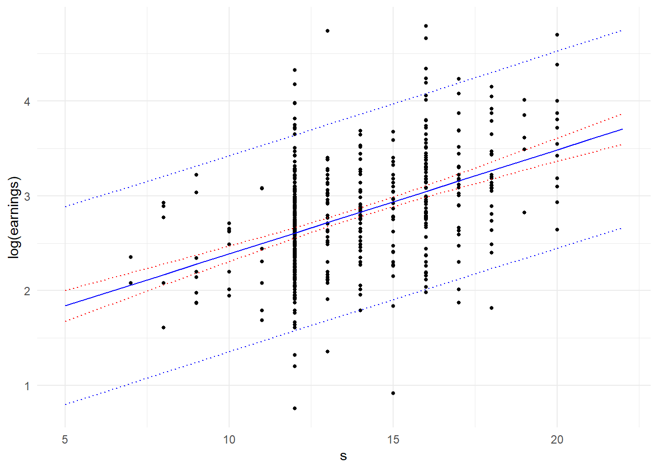
Fig. 5.3 presents several interesting questions. Suppose we were interested in predicting a new observation at \(s=16\). In our data set we have several (in fact 88) observations at \(s=16\). Would it make sense to simply use the sample mean of those 88 observations as our prediction? You would still get unbiased estimators, although your prediction would be based on only 88 observations, and in situations where you have very few observations at a certain s, your prediction and estimates of the MSPE can be unreliable. On the other hand, if indeed the conditional expectation of log(earnings) is a linear function of s, then we can use the entire data set to estimate just two parameters which would reduce sampling errors considerably.
Nonetheless, using just the observations at s=16 might actually be a sensible thing to do if we were very unsure about the form of the conditional expectation. If the conditional expectation is non-linear, then the linear regression line would only be an approximation (possibly a very poor one) and would give biased predictions. The sample mean at s=16 would be unbiased, though it would have greater variance.
What we have is a bias-variance trade-off. If the conditional expectation is non-linear, but only slightly, then imposing the assumption would result in slightly biased predictions, but we would be able to draw on the whole data set to reduce sampling error. It may be the case that allowing for a slight bias might reduce variance sufficiently to reduce mean squared error, which is variance plus squared bias.
Another question: Why are we predicting log(earnings) and not earnings? Probably it is the latter that we want, but the relationship between earnings and s is definitely not linear, see Fig. 5.4
ggplot() +
  geom_point(data=df_earn,aes(x=s, y=earnings), size=1)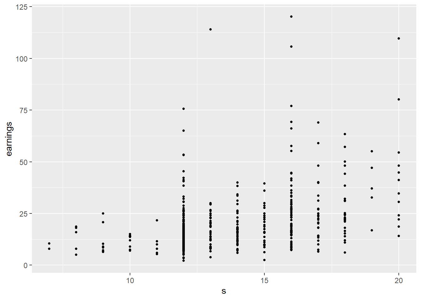
We may be able to effectively model such non-linearity using a multiple linear regression framework, but often a simple transformation of one or more of the variables works well to linearize a relationship. As we see in Fig. 5.3, a linear relationship between log(earnings) and s is not entirely unreasonable, and using log(earnings) also alleviates some of the heteroskedasticity issues that we see in Fig. 5.4.
But then, how do we convert a prediction of \(\log Y\) to a prediction of \(Y\)? One way would be to simply reverse the log() transformation, and use \[
\exp(\widehat{\log Y})
\] as the prediction. However, \(\widehat{\log y}\) is an estimate of \(E[\log Y | X]\), and because \(\exp()\) is a convex function, \[
\exp E[\log Y | X] \leq E[\exp \log Y | X]
\] In other words we would be systematically under-estimating \(E[\log Y|X]\).
We know that if \(\log Y \sim \text{Normal}(\mu, \sigma^2)\), then \(Y\) has the log-normal distribution with mean \[ E[Y] = \exp (\mu) \exp(\sigma^{2}/2)\,. \] If we assume normality of the error terms in the log-regression, i.e., \[ \log Y = \beta_{0} + \beta_{1} X + \epsilon\,,\,\,\epsilon \sim \text{Normal}(0,\sigma^{2})\,, \] then \[ (\log Y) | X \sim \text{Normal}(\beta_{0} + \beta_{1} X, \sigma^{2}) \] which means \[ E[Y|X] = \exp (\beta_{0} + \beta_{1} X) \exp(\sigma^{2}/2)\,. \] This suggests using the transformation \[ \exp(\widehat{\log Y})\exp\left(\frac{\widehat{\sigma^{2}}}{2}\right) \] to convert predictions of \(\log Y\) to predictions of \(Y\).
5.4 Hypothesis Testing
We often want to test if \(\beta_1\) is equal to some value in population. For instance, is the price elasticity of a product equal to 1? This would be the hypothesis \(H_0: \beta_1=1 \text{ vs } H_A: \beta_1 \neq 1\) in the regression \[ \ln Y_{i} = \beta_{0} + \beta_{1} \ln X_{i} + \epsilon_{i} \] where \(X\) is the price and \(Y\) is quantity sold. We call \(H_{0}\) the “null hypothesis” and \(H_{A}\) the “alternative hypothesis”. Is a job training program effective? This would be the hypothesis \(H_0: \beta_1=0 \text{ vs } H_A: \beta_1 \neq 0\) in the regression \[ Y = \beta_{0} + \beta_{1} X + \epsilon_{i}\,. \] where \(X\) is an indicator of participation in a job training program and \(Y\) is some outcome variable.
The basic strategy for checking if \(\beta_1\) is equal to some value \(\beta_1^*\) in population is to check if \(\hat{\beta}_1\) is “improbably far” from \(\beta_1^*\), given what we know about the distribution of \(\hat{\beta}_1\) “under the null”, i.e., when \(\beta_1 = \beta_1^*\). In order to derive this distribution, at least in finite samples, we have to make an addition assumption regarding the conditional distribution of \(\epsilon\). If we assume that
(A6) \(\epsilon | X \sim \mathrm{Normal}(0,\sigma^2)\)
then under random sampling, we will have \[ \epsilon_i | X_1,X_2,\dots,X_N \; \sim \; \mathrm{Normal}(0,\sigma^2). \] Under the null hypothesis we have \[ \hat{\beta}_1 = \beta_1^* + {\sum_{i=1}^N w_i\epsilon_i}. \] Since \(\hat{\beta}_1\) is a constant plus a linear combination of normally distributed terms, it is normally distributed (conditional on \(\{X_1,X_2,\dots,X_N\}\)). We have already shown that \(E[\hat{\beta}_1|X_1,...,X_N]\) is unbiased and \(var[\hat{\beta}_1|X_1,...,X_N]= \sigma^2/\sum_{i=1}^N(X_i-\overline{X})^2\). Therefore under the null hypothesis that \(\beta_1 = \beta_1^*\) we have \[ \hat{\beta}_1|X_1,...,X_N \sim \text{Normal}\left(\beta_1^*, \frac{\sigma^2}{\sum_{i=1}^N(X_i-\overline{X})^2}\right). \] That is, \[ \left.\frac{\hat{\beta}_1-\beta_1^*}{\sqrt{\frac{\sigma^2}{\sum_{i=1}^N(X_i-\overline{X})^2}}} \right|X_1,...,X_N \; \sim \; \text{Normal}(0, 1). \] The remaining problem is that \(\sigma^2\) is unknown. It turns out that replacing \(\sigma^2\) with \(\widehat{\sigma^2}\) as calculated in Eq. 5.17, we have \[ t = \frac{\hat{\beta}_1-\beta_1^*}{\sqrt{\frac{\widehat{\sigma^2}}{\sum_{i=1}^N(X_i-\overline{X})^2}}} \; \sim \; t_{(N-2)}. \tag{5.23}\] We can drop the conditioning information, since the t-distribution does not depend on \(X_1,...,X_N\). In other words, the result holds unconditionally.
We can then use Eq. 5.23 to test \(H_0: \beta_1=\beta_1^*\) in the usual way. For instance, for a 0.05 test, we can use the rule “reject \(H_0: \beta_1=\beta_1^*\) if the absolute value of \(t\) in Eq. 5.23 exceeds \(t_{0.025,N-2}\) where \(t_{0.025,N-2}\) is the \(0.975\) percentile of the \(t_{N-2}\) distribution. The denominator is just the square root of the usual estimator of \(var[\hat{\beta}_1]\). If we are testing if \(\beta_1=0\), then Eq. 5.23 is just the parameter estimate divided by its standard error.
Example 5.5 We continue with Example 5.2, where we fit the regression \(Y_{i} = \beta_{0} + \beta_{1} X_{i} + \epsilon_{i}\) on a simulated dataset with \(N=10\) observations, and obtained the estimates
cat("beta1hat = ", round(b1hat,3), "\n")
cat("s.e.(beta1hat) = ", round(sqrt(estvarb1hat),3), "\n")
beta1hat = 0.908
s.e.(beta1hat) = 0.42 Suppose we are interested in testing the hypothesis \(H_{0}: \beta_{1} = 0\) vs the usual two-sided alternative, then the appropriate t-statistic is
t1 = b1hat / sqrt(estvarb1hat)
cat("t-stat(beta1=0) = ", round(t1,3))
t-stat(beta1=0) = 2.162The critical value for the test at 0.01, 0.05 and 0.10 levels of significance is
round(c("0.10" = qt(0.95, 8), "0.05" = qt(0.975, 8), "0.01" = qt(0.995, 8)), 3) 0.10 0.05 0.01
1.860 2.306 3.355 We reject the hypothesis at 0.10 significance level, but not at 0.01 and 0.05 significance levels. Alternatively, we can compute the p-value for this test.
cat("p-val (b1=0) is: ", round((1-pt(abs(t1), 8))*2,4), "\n")p-val (b1=0) is: 0.0626 To test \(H_{0}: \beta_{1} = 1 \text{ vs } H_{A}: \beta_{1} \neq 1\), the t-statistic is
t2 = (b1hat-1) / sqrt(estvarb1hat)
cat("t-stat(beta1=1) = ", round(t2,3), "with p-value: ", round((1-pt(abs(t2), 8))*2,4), "\n")
t-stat(beta1=1) = -0.22 with p-value: 0.8317 We do not reject this test at any of the usual significance levels.
Most of the calculations here can be obtained via R’s lm() function:
mdl <- lm(Y~X, data=df)
mdl_sum <- summary(mdl)
print(mdl_sum)
Call:
lm(formula = Y ~ X, data = df)

Residuals:
    Min      1Q  Median      3Q     Max
-5.2180 -2.3236  0.8198  1.5689  4.3465

Coefficients:
            Estimate Std. Error t value Pr(>|t|)
(Intercept)   4.3473     1.9658   2.211   0.0580 .
X             0.9078     0.4200   2.162   0.0626 .
---
Signif. codes:  0 '***' 0.001 '**' 0.01 '*' 0.05 '.' 0.1 ' ' 1

Residual standard error: 3.138 on 8 degrees of freedom
Multiple R-squared:  0.3687,    Adjusted R-squared:  0.2898
F-statistic: 4.673 on 1 and 8 DF,  p-value: 0.06262
The t-values reported are just the estimate divided by the standard error, and can be used to test (separately) the hypotheses \(\beta_0=0\) and \(\beta_1=0\). The p-values indicate that we reject these hypotheses at 10%, but not at 5%. Since this is simulated data with both parameters set at \(\beta_0=4\) and \(\beta_1=1.5\), we know that we make the wrong inference (we do not reject a false hypothesis) with the 0.05 and 0.01 tests. There is always the possibility of non-rejection of a false hypothesis, but in this case, this is due to the small sample size and relatively noisy data, leading to relatively large standard errors, and small t-values. For the test \(H_{0}: \beta_{1} = 1 \text{ vs } H_{A}: \beta_{1} \neq 1\) you can use the linearHypothesis() function from the car package. The test reported is an “F-test” and not a t-test, although for tests of a single restriction they are equivalent (notice that the p-value is identical to the t-test reported previously for this hypothesis). We will discuss the F-test in a later chapter.
car::linearHypothesis(mdl, "X=1")Linear hypothesis test
Hypothesis:
X = 1
Model 1: restricted model
Model 2: Y ~ X
Res.Df RSS Df Sum of Sq F Pr(>F)
1 9 79.269
2 8 78.794 1 0.4746 0.0482 0.83175.5 Asymptotic Results
The results obtained so far are “finite sample” results, i.e., are valid for any given sample size \(N\) (when Assumption Set A holds). The OLS estimators also have good properties in the limit as \(N \rightarrow \infty\), or “asymptotically”. We continue to focus of \(\hat{\beta}_1\).
Consistency \(\hat{\beta}_1 \rightarrow_p \beta_1\).
The starting point for showing this result is Eq. 5.11 which we restate here, expanding \(w_i\) and dividing the numerator and denominator of the last term by \(1/N\): \[ \begin{aligned} \hat{\beta}_1 & = \beta_1 + \sum_{i=1}^N w_i\epsilon_i \\ & = \beta_1 + \frac{(1/N)\sum_{i=1}^N (X_i-\overline{X})\epsilon_i}{(1/N)\sum_{i=1}^N (X_i-\overline{X})^2} \,. \end{aligned} \tag{5.24}\] The last term is the ratio of sample covariance of \(X_i\) and \(\epsilon_i\) to the sample variance of \(X_i\). If we assume that the conditions are such that the sample covariance of \(X_i\) and \(\epsilon_i\) converges in probability to the population covariance of \(X\) and \(\epsilon\), and likewise that the sample variance of \(X_i\) converges in probability to the population variance of \(X\), and that the population variance of \(X\) is not zero, then \[ \hat{\beta}_1 = \beta_1 + \frac{\overbrace{(1/N)\sum_{i=1}^N (X_i-\overline{X})\epsilon_i}^{\rightarrow_p \, \mathrm{cov}[X,\epsilon]=0}} {\underbrace{(1/N)\sum_{i=1}^N (X_i-\overline{X})^2}_{\rightarrow_p \, var[X]\neq0}} \rightarrow_p \beta_1 \tag{5.25}\] The assumption that \(\mathrm{cov}[X,\epsilon]=0\) comes directly from the assumption that \(E[\epsilon|X]=0\). Earlier we assumed that \(\sum_{i=1}^N (X_i-\overline{X})^2 \neq 0\). We modify this assumption slightly to \(var[X] \neq 0\) (as noted earlier, the former is implied by the latter and random sampling). Convergence in probability comes about from the laws of large numbers. Earlier we stated the LLN as the convergence in probability of a sample mean to the population mean. The covariance of \(X\) and \(\epsilon\) is a population expectation (of the random variable \((X-E[X])(\epsilon-E[\epsilon])\)) and the sample covariance of \(X_i\) and \(\epsilon_i\) is a sample average of observations of this random variable. Likewise, for the sample variance in the denominator. As long as the conditions for the LLN hold for these sample means, convergence in probability will follow.
It can be shown that under a mild extension of Assumption Set A, we have \[ \sqrt{N}(\hat{\beta}_1 - \beta_1) \rightarrow_d \text{Normal}\left(0,\frac{\sigma^2}{var[X]}\right) \tag{5.26}\] or \[ \frac{\sqrt{N}(\hat{\beta}_1 - \beta_1)}{\sqrt{\sigma^2/var[X]}} \rightarrow_d \text{Normal}(0,1)\,. \]
We can replace \(\sigma^2\) and \(E[X]\) with consistent estimates of the two. Replacing \(\sigma^2\) with \(\widehat{\sigma^2}\) and using \((1/N)\sum_{i=1}^N(X_i-\overline{X})^2\) as a consistent estimator for \(var[X]\), we have \[ \frac{\hat{\beta}_1 - \beta_1}{\sqrt{\frac{\widehat{\sigma^2}}{\sum_{i=1}^N(X_i-\overline{X})^2}}} \rightarrow_d \text{Normal}(0,1). \] The left hand side is just the t-statistic in Eq. 5.23. In other words, we can continue to use the t-statistic, but we choose the rejection region from the standard normal distribution rather than the t-distribution. This test would only be approximate, but if the sample size is large enough it should be sufficiently accurate.
We omit details of the proof of Eq. 5.26, but the intuition is as follows: write \[ \begin{aligned} \hat{\beta}_1 &= \beta_1 + \sum_{i=1}^N w_i \epsilon_i \\ &= \beta_1 + \left[\frac{1}{N}\sum_{i=1}(X_i-\overline{X})^2\right]^{-1} \frac{1}{N}\sum_{i=1}(X_i-\overline{X})\epsilon_i \end{aligned} \] or \[ \begin{aligned} \sqrt{N}(\hat{\beta}_1-\beta_1) &= \left[\frac{1}{N}\sum_{i=1}^N(X_i-\overline{X})^2\right]^{-1} \frac{1}{\sqrt{N}}\sum_{i=1}^N(X_i-\overline{X})\epsilon_i \\ &= \left[\frac{1}{N}\sum_{i=1}^N(X_i-\overline{X})^2\right]^{-1} \frac{1}{\sqrt{N}}\sum_{i=1}^Nb_i\epsilon_i \end{aligned} \] where \(b_i = X_i - \overline{X}\). The random variables \(\{b_i\epsilon_i\}_{i=1}^N\) have mean \[ E[b_i\epsilon_i] = E[E[b_i\epsilon_i|X_1,...,X_N]] = E[b_iE[\epsilon_i|X_1,...,X_N]] = 0 \] and variance \[ E[(b_i\epsilon_i)^2] = E[b_i^2E[\epsilon_i^2|X_1,...,X_N]] = \sigma^2E[b_i^2]. \] If the required conditions for a relevant CLT hold, we have \[ \frac{1}{\sqrt{N}}\sum_{i=1}^Nb_i\epsilon_i \rightarrow_d N(0,\sigma^2E[b_i^2])\,. \] Since \((1/N)\sum_{i=1}^N (X_i - \overline{X})^2 \rightarrow_p var[X]\), evidently \(E[b_i^2]\) is \(var[X]\). Therefore \[ \begin{aligned} \sqrt{N}(\hat{\beta}_1-\beta_1) &= \overbrace{\left[\frac{1}{N}\sum_{i=1}^N(X_i-\overline{X})^2\right]^{-1}} ^{\rightarrow_p \; var[X]^{-1}} \overbrace{\quad\frac{1}{\sqrt{N}}\sum_{i=1}^Nb_i\epsilon_i\quad} ^{\rightarrow_d \; \mathrm{Normal}(0,\sigma^2 var[X])}\\ \;&\\ &\rightarrow_d \; \mathrm{Normal}(0,\sigma^2var[X]^{-1}) \end{aligned} \]
5.6 When Baseline Assumptions are Violated
In summary, OLS estimation behaves well when Assumption Set A holds. What happens if one or more of the assumptions fail to hold?
5.6.1 Heteroskedasticity
The assumption of conditional homoskedasticity is that the variance of the noise terms do not depend on the regressors. The proof of unbiasedness (and consistency) of OLS estimators did not use this assumption in any way, which implies that violation of conditional homoskedasticity (such as in Example 5.1) does not affect unbiasedness. However, the derivation of the formulas for \(var[\hat{\beta}_{1}]\) and \(var[\hat{\beta}_{0}]\) do use this assumption, so the derived formulas for the estimator variances and t-tests are incorrect when conditional homoskedasticity fails to hold. Estimator variances computed using the formulas derived under homoskedasticity when the noise terms are heteroskedastic are unreliable. Furthermore, it turns out that OLS is no longer minimum variance among unbiased linear estimators, i.e., OLS is no longer “efficient”. Discussions about how OLS should be amended in response to conditional heteroskedasticity will have to wait until a later chapter, when we discuss heteroskedasticity in more detail.
5.6.2 Endogeneity
Recall that one of the key assumptions for unbiasedness of OLS estimators is that \(E[\epsilon_{i} | X_{1}, \dots, X_{N}] = 0\). This assumption may fail to hold if \(E[\epsilon | X] = 0\) does not hold in population, or if there are sampling issues. “Endogeneity” is the word used to describe such situations.
Example 5.6 (Truncated Sampling) Suppose \(\beta_1\) is positive so you have a positively sloped PRF. Suppose you have a “truncated sample” where you cannot observe any observation where \(Y_i > c\). This means that the only observations with larger values of \(X_i\) that are included in your sample will be the ones with lower or negative values of \(\epsilon_i\), since a large \(X_i\) together with large positive \(\epsilon_i\) makes \(Y_i>c\) more likely. This implies a negative correlation between \(X\) and \(\epsilon\), and invalidates the assumption \(E[\epsilon_{i} | X_{1}, \dots, X_{N}]=0\). The following is an empirical illustration where the PRF has a positive slope, and observations with \(Y_i>1500\) are unavailable. The plot in Fig. 5.5 shows the full (black circles) and truncated (red x’s) samples. The estimated OLS sample regression line for the full data set (black) and the truncated data set (red) are shown, illustrating the downward bias in \(\hat{\beta}_{1}\).
  set.seed(13)
  X <- rnorm(100, mean=50, sd=20)
  Y <- 1220 + 4*X + rnorm(100, mean=0, sd=50)
  df_notrunc <- data.frame(X, Y)
  df_trunc <- filter(df_notrunc, Y<=1500)
  ggplot() +
    geom_point(data=df_notrunc,aes(x=X,y=Y), pch=1, size=2) +
    geom_smooth(data=df_notrunc,aes(x=X,y=Y), method="lm", se=FALSE, col="black") +
    geom_point(data=df_trunc, aes(x=X,y=Y), pch=4, size=2,col='red') +
    geom_smooth(data=df_trunc,aes(x=X,y=Y), method="lm", se=FALSE, col="red") +
    theme_minimal()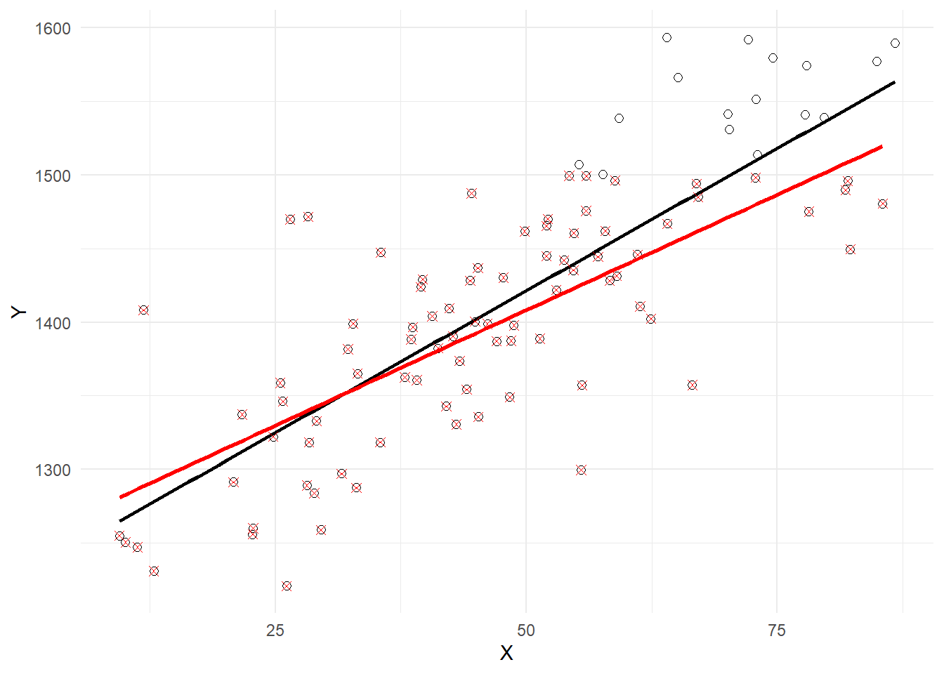
Example 5.7 (Measurement Error) Another kind of sampling issue is measurement error. Suppose \(Y = \beta_0 + \beta_1 X + \epsilon\) describes the relationship between \(Y\) and \(X\), but \(X\) is only observed with error, i.e., you observe \(X^{*} = X + u\). Assume that the measurement error \(u\) is independent of \(X\). Then \[ \begin{aligned} Y &= \beta_0 + \beta_1 X + \epsilon \\ &= \beta_0 + \beta_1 (X^* - u) + \epsilon \\ &= \beta_0 + \beta_1 X^* + (\epsilon - \beta_1u) \\ &= \beta_0 + \beta_1 X^* + v \end{aligned} \] where \(v = \epsilon - \beta_1 u\). You proceed with what appears to be the only feasible option to you, which is to run the regression \[ Y = \beta_0 + \beta_1 X^* + v\,, \] but since \(u\) is correlated with \(X^*\), the assumption \(E[v|X^*]=0\) does not hold. In the simulated example below, we have a positively sloped PRF, shown in red, and measurement error in the regressor. Since \(\beta_1\) is positive, \(X^*\) and \(v\) are negatively correlated, meaning that the error term \(v\) will tend to be positive for smaller \(X*\) and negative for larger \(X*\). This tendency is visible in Fig. 5.6 below. The red circles are the sample you would have observed with no measurement error. The black circles are the same sample points, but with measurement error in the \(X_{i}\)’s.
  set.seed(13)
  X <- rnorm(100, mean=50, sd=20)
  Y <- 1220 + 4*X + rnorm(100, mean=0, sd=10)
  Xstar <- X + rnorm(100, mean=0, sd=10)
  df_measerr <- data.frame(X, Y, Xstar)
  ggplot() +
    geom_point(data=df_measerr,aes(x=Xstar,y=Y), pch=1, size=2) +
    geom_point(data=df_measerr,aes(x=X,y=Y), pch=1, size=2, col="red") +
    geom_abline(intercept=1220, slope=4, col='red') +
    geom_smooth(data=df_measerr, aes(x=Xstar, y=Y), method="lm", col='black',
                se=FALSE, linewidth=0.8) + xlab("X, Xstar") +
    theme_minimal()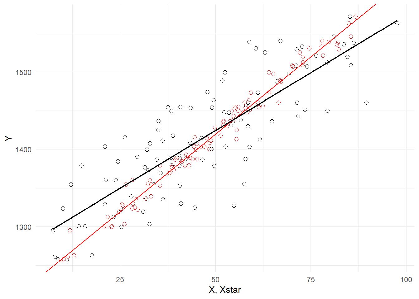
Example 5.8 (Simultaneity Bias) Suppose the market for a good is governed by the following demand and supply equations \[ \begin{aligned} Q_t^d &= \delta_0 + \delta_1 P_t + \epsilon_t^d \hspace{1cm} &(\text{Demand Eq } \delta_1 < 0) \\ Q_t^s &= \alpha_0 + \alpha_1 P_t + \epsilon_t^s \hspace{1cm} &(\text{Supply Eq } \alpha_1 > 0) \\ Q_t^s &= Q_t^d \hspace{3cm} &(\text{Market Clearing}) \end{aligned} \] where \(Q\) and \(P\) represent log quantities and log prices respectively, so \(\delta_1\) and \(\alpha_1\) represent price elasticities of demand and supply respectively. Suppose the demand shock \(\epsilon_t^d\) and supply shock \(\epsilon_y^s\) are iid noise terms with zero means and variances \(\sigma_d^2\) and \(\sigma_s^2\) respectively, and are mutually uncorrelated. Market clearing means that observed quantity and prices occur at the intersection of the demand and supply equations, i.e., observed quantity and prices are such that \[ \delta_0 + \delta_1 P_t + \epsilon_t^d = \alpha_0 + \alpha_1 P_t + \epsilon_t^s\,. \] which we can solve to get \[ P_t = \frac{\alpha_0 - \delta_0}{\delta_1 - \alpha_1} + \frac{\epsilon_t^s - \epsilon_t^d}{\delta_1 - \alpha_1}. \tag{5.27}\] Substituting this expression for prices into either the demand or supply equation gives \[ Q_t = \left(\delta_0 + \delta_1\frac{\alpha_0 - \delta_0}{\delta_1 - \alpha_1}\right) + \frac{\delta_1\epsilon_t^s - \alpha_1\epsilon_t^d}{\delta_1 - \alpha_1}\,. \tag{5.28}\] Equations Eq. 5.27 and Eq. 5.28 imply \[ var[P_t] = \frac{\sigma_s^2 + \sigma_d^2}{(\delta_1 - \alpha_1)^2} \quad \text{ and } \quad \mathrm{cov}[P_t, Q_t] = \frac{\delta_1\sigma_s^2 + \alpha_1\sigma_d^2}{(\delta_1 - \alpha_1)^2}. \] This means that in a regression of \(Q_t = \beta_0 + \beta_1 P_t + \epsilon_t\), we will get \[ \hat{\beta}_1 \rightarrow_p \frac{\mathrm{cov}[Q_t, P_t]}{var[P_t]} =\frac{\delta_1\sigma_s^2 + \alpha_1\sigma_d^2}{\sigma_s^2 + \sigma_d^2} \] which is neither the price elasticity of demand nor the price elasticity of supply.
The problem in this example is that prices and quantities are simultaneously determined by the intersection of the demand and supply functions; both prices and quantities are “endogenous” variables. The consequence of this is that regardless of whether you view the regression of \(Q_t\) on \(P_t\) as estimating the demand or supply equation, the noise term in the regression will be correlated with \(P_t\). A supply shock shifts the supply function and changes both \(Q_t\) and \(P_t\). Likewise, a demand shock shifts the demand function and again changes both \(Q_t\) and \(P_t\). The use of the term “endogeneity” comes from applications like these, but it is now used for all situations where the noise term is correlated with one or more of the regressors.
Example 5.9 (Omitted Variables) Suppose \(X\) and \(Z\) are “causal” variables for \(Y\), and we wish to measure the effect \(X\) has on \(Y\). Suppose \[ Y = \alpha_0 + \alpha_1 X + \alpha_2 Z + w \tag{5.29}\] where \(\alpha_2 \neq 0\) and \(E[w|X,Z]=0\). That is, \[ E[Y|X,Z] = \alpha_0 + \alpha_1 X + \alpha_2 Z. \] If we omit \(Z\) from Eq. 5.29 and write it as \[ Y = \alpha_0 + \alpha_1 X + \epsilon \] we would be subsuming the variable \(Z\) into the noise term \(\epsilon\) \[ \epsilon = \alpha_2 Z + w. \] If \(X\) and \(Z\) are correlated, then \(\mathrm{cov}[X,\epsilon] \neq 0\). In a regression of \(Y\) on \(X\), the OLS estimator \(\hat{\alpha}_1\) will be biased and inconsistent for \(\alpha_1\). We have not specified enough detail to derive an expression for the bias, but it is easy to show inconsistency. The OLS estimator for \(\hat{\alpha}_1\) is \[ \hat{\alpha}_1 = \alpha_1 + \frac{\sum_{i=1}^N(X_i-\overline{X})\epsilon_i}{\sum_{i=1}^N(X_i-\overline{X})^2} \] which will converge in probability to \[ \alpha_1 + \frac{\mathrm{cov}[X,\epsilon]}{var[X]} \neq \alpha_1. \] That is, the OLS estimator \(\hat{\alpha}_1\) will be inconsistent for \(\alpha_1\) and will misrepresent the degree of causality from \(X\) to \(Y\).
The following is a more detailed example of a situation described in Example 5.9
Example 5.10 Suppose the true relationship of the variables \(X\), \(Y\) and \(Z\) is given by \[ \begin{gathered} Y = \alpha_0 + \alpha_1 Z + u \\ X = Z + v \end{gathered} \tag{5.30}\] That is, both \(Y\) and \(X\) are driven by a third variable \(Z\) but are otherwise not connected. Assume the noise terms \(u\) and \(v\) are independent of each other, with \(u \sim N(0, \sigma_u^2)\) and \(v \sim N(0,\sigma_v^2)\). Suppose also that \(Z \sim N(0,\sigma_Z^2)\). In this example, there are in fact values \(\beta_0\) and \(\beta_1\) such that assumptions A1 to A3 in assumption set A hold. It can be shown (see exercises) that \[ E[Z|X] = \frac{\sigma_Z^2}{\sigma_Z^2 + \sigma_v^2}X. \tag{5.31}\] (Intuition for Eq. 5.31 : \(Z\) obviously has information about \(X\), but given \(X\) one also gets information about \(Z\). If \(\sigma_v^2=0\) obviously \(Z=X\). On the other hand, if \(\sigma_v^2\) is very large, then the information content in \(X\) about \(Z\) is small, and the expected value should be close to the unconditional mean of \(Z\) which is zero.) From Eq. 5.31, we get \[ E[Y|X] = \alpha_0 + \alpha_1E[Z|X] + E[u|X] = \alpha_0 + \frac{\alpha_1\sigma_Z^2}{\sigma_Z^2 + \sigma_v^2}X. \tag{5.32}\] It follows that \(E[\epsilon|X]=0\) where \(\epsilon = Y - \beta_0 - \beta_1X\) with \(\beta_0=\alpha_0\) and \(\beta_1 = \frac{\alpha_1\sigma_Z^2}{\sigma_Z^2 + \sigma_v^2}\). It is also straightforward to show that the conditional variance is a constant.
Since Assumption Set A holds, OLS estimation of a regression of \(Y_i\) on \(X_i\) will produce an unbiased and consistent estimator for \(\beta_1\), but this non-zero \(\beta_1\) does not indicate causality of \(X\) on \(Y\). In this example, it is \(Z\) that drives both \(Y\) and \(X\). Any movements in \(X\) resulting from \(v\) but not \(Z\) will not result in any response in \(Y\). But because \(Z\) drives both \(X\) and \(Y\), one will observe a correlation between \(X\) and \(Y\).
The next example is an illustration of the previous two examples.
Example 5.11 We use the data in earnings.xlsx for this example. This data set contains a sample of 540 individuals with information including earnings, height, sex, years of schooling, among other variables. We run a regression of \(\ln(earnings)\) on \(height\).
df_cause <- read_csv("data\\earnings.csv")
mdl_cause <- lm(log(earnings)~height, data=df_cause)
summary(mdl_cause)
Call:
lm(formula = log(earnings) ~ height, data = df_cause)

Residuals:
     Min       1Q   Median       3Q      Max
-2.21599 -0.37662 -0.01233  0.33506  2.06550

Coefficients:
            Estimate Std. Error t value Pr(>|t|)
(Intercept) 0.026104   0.387961   0.067    0.946
height      0.040871   0.005722   7.143 2.98e-12 ***
---
Signif. codes:  0 '***' 0.001 '**' 0.01 '*' 0.05 '.' 0.1 ' ' 1

Residual standard error: 0.563 on 538 degrees of freedom
Multiple R-squared:  0.08663,   Adjusted R-squared:  0.08493
F-statistic: 51.03 on 1 and 538 DF,  p-value: 2.976e-12
We find that the effect of \(height\) on \(\ln(earnings)\) is statistically significant (and economically significant at 4% per inch), and “explains” over 8.6% of the variation in \(ln(earnings)\). However, all this seems unlikely to be a true indication of “causality” in the sense of height causing earnings, ceteris paribus. In particular, the sample includes observations on both males and females. The result most likely reflects the wage gap between males and females. This is picked up by \(height\) since there is also a systematic difference in the heights of males and females.
One of the main applications of regression analysis is to empirically explore if one variable causes another, or at least the extent to which one variable causes another. However, what simple linear regression captures is correlation between two variables, and correlation does not necessarily reflect causality.
The ideal scenario for measuring causation of \(X\) to \(Y\) would be to literally hold everything else fixed, change \(X\), and see how \(Y\) changes, but this is obviously impossible to do here. In some applications we may be able to sample in such a way so that the noise \(\epsilon\) is uncorrelated with \(X\) by construction (this is the approach of randomized controlled trials). With observational data, we have to find some other way to ‘control’ for confounding factors.
The solution to the omitted variable problem is (wherever possible) to include all relevant explanatory variables into the regression. This takes us to the multiple linear regression framework, which we cover in the next chapter. The solution to the other endogeneity problems require more advanced techniques.
5.7 Exercises
Exercise 5.1 What is the OLS estimator for \(\beta_0\) in the linear regression model with no regressor, i.e., in the regression \(Y_i = \beta_0 + \epsilon_i\)? What is the \(R^2\) for this regression?
Remark: All of our regressions will include the intercept term, unless explicitly stated otherwise.
Exercise 5.2 You should have found the \(\hat{\beta}_0\) in Exercise 5.1 to be the sample mean \(\overline{Y}\). Suppose you choose to estimate \(\beta_0\) using some other measure of location (perhaps the median of \(Y_i\)). What can you say about the \(R^2\) in this case?
Exercise 5.3 Show for the simple linear regression model (with intercept term included) that the \(R^2\) is the square of the correlation coefficient of \(Y_i\) and \(\hat{Y}_i\), i.e., \[ R^2 = \left[\; \frac{\sum_{i=1}^N(Y_i - \overline{Y})(\hat{Y}_i - \overline{\hat{Y}})} {\sqrt{\sum_{i=1}^N(Y_i - \overline{Y})^2}\sqrt{\sum_{i=1}^N(\hat{Y}_i - \overline{\hat{Y}})^2}} \; \right]^2 \] This is where the name “\(R^2\)” comes from. Show also that \[ R^2 = \left[\; \frac{\sum_{i=1}^N(Y_i - \overline{Y})(X_i - \overline{X})} {\sqrt{\sum_{i=1}^N(Y_i - \overline{Y})^2}\sqrt{\sum_{i=1}^N(X_i - \overline{X})^2}}. \; \right]^2 \] The first of these two expressions will hold for OLS estimation of the multiple linear regression model. The second is specific to the simple linear regression model.
Exercise 5.4 Explain why \(\sum_{i=1}^N w_iv_i = 0\) in Eq. 5.20.
Exercise 5.5 Show that \(E[Z|X] = \frac{\sigma_Z^2}{\sigma_Z^2 + \sigma_v^2}X\) in Example 5.9). (Hint: Look up the notes on the Bivariate Normal Distribution.)
Exercise 5.6 Show for the simple linear regression (with intercept) that any observation \((X_i,Y_i)\) such that \(X_i = \overline{X}\) does not numerically affect the value of the OLS estimator \(\hat{\beta}_1\).
Exercise 5.7 Suppose we wish to estimate a simple linear regression on a data set \(\{X_i,Y_i\}_{i=1}^{80}\), but because of a clerical error, twenty additional rows of zeros were added to the excel file containing the data. That is, instead of estimating the regression on \(\{X_i,Y_i\}_{i=1}^{80}\), the regression was estimated on \(\{X_i,Y_i\}_{i=1}^{100}\) where \((X_i,Y_i) = (0,0)\) for \(i=81,...,100\). Explain why this error does not affect the numerical value of \(\hat{\beta}_1\). Will it affect the numerical value of \(\hat{\beta_0}\)? What about their variances?
Exercise 5.8 Suppose you have a data set \(\{X_i,Y_i\}_{i=1}^N\) where \(X_i\) is binary, with \(N_0\) observations where \(X_i=0\) and \(N_1\) observations where \(X_i=1\), \(N_0 + N_1 = N\). You estimate a simple linear regression model on this data set using OLS. Show that \(\hat{\beta}_0\) is equal to the sample mean of \(Y_i\) over all observations where \(X_i=0\), i.e., \(\hat{\beta}_0=(1/N_0)\sum_{i:X_i=0}Y_i\) and \(\hat{\beta}_1\) is equal to the sample mean of \(Y_i\) over all observations where \(X_i=1\) minus the sample mean of \(Y_i\) over all observations where \(X_i=0\), i.e., \[ \hat{\beta}_1=\frac{1}{N_1}\sum_{i:X_i=1}Y_i - \frac{1}{N_0}\sum_{i:X_i=0}Y_i. \]
Exercise 5.9 We have shown that measurement error in the regressor leads to inconsistent estimators. Does measurement error in the regressand \(Y\) also result in inconsistent estimators?
Exercise 5.10 The data set Anscombe.xlsx contains for four pairs of variables: \((X1,Y1)\), \((X2,Y2)\), \((X3,Y3)\) and \((X4,Y4)\).
Regress \(Y1\) on \(X1\), \(Y2\) on \(X2\), \(Y3\) on \(X3\) and \(Y4\) on \(X4\) in four separate regressions (all with intercept term). Report the results as given in
coef(summary()), and the \(R^2\) for all four regressions. What do you observe? For each regression, plot the data and the fitted SRF in one diagram (one figure per regression) and plot the residuals against the regressors in a separate diagram (also one each per regression), and comment on the plots. This exercise shows you the important of visually inspecting your regressions.For each of the four regressions in part (a), verify that the residuals sum to zero and are orthogonal to the regressor.
Exercise 5.11 Derive Eq. 5.22.
Exercise 5.12 Refer to the earnings.csv data set which contains observations of a sample of adult workers. The variable earnings is hourly earnings and age is the age of workers. Consider the regression \[
log(earnings) = \beta_{0} + \beta_{1} age + \epsilon\,.
\] a. What is the interpretation of \(\beta_{1}\)? b. Does \(\beta_{0}\) have an economic interpretation? c. What would be the interpretation of \(\beta_{0}\) be in the regression \[
log(earnings) = \beta_{0} + \beta_{1} (age-21) + \epsilon\,?
\]
The “-scedasticity” part of the words homoskedasticity and heteroskedasticity come from an ancient greek word that can be translated to “scatter”. “Homo-” and “Hetero-” come from words translating to “equal” and “different” respectively.↩︎
Sometimes the word “explained” is used instead.↩︎
Our simulation experiment actually illustrates “conditional unbiasedness” as in Eq. 5.15. To show “unconditional unbiasedness” in the simulation experiment, move the line
X <- rnorm(10, mean=5, sd=2)from just above theforstatement to just below it (i.e., to just aboveY <- 2 + 1.5*X + rnorm(10, mean=0, sd=3)).↩︎