2  Miscellaneous Mathematics Topics

We briefly review some math prerequisites, specifically: how to use the summation notation, an introduction to matrices, and a little optimization theory. We follow up on matrix algebra in later chapters. The R code uses the tidyverse and patchwork libraries.

library(tidyverse)
library(patchwork)  # for laying out plots

2.1 The Summation Notation

We use the uppercase sigma “\(\Sigma\)” in the following way to denote summation. For a set of numbers \(\{x_1,x_2,...,x_n\}\), define \[ \sum_{i=1}^n x_i = x_1+x_2+...+x_n. \]

Example 2.1 The sample mean of a set of numbers \(\{x_1,x_2,...,x_n\}\) is \[ \overline{x}= \frac{1}{n}\sum_{i=1}^n x_i\;. \]

Example 2.2 Write \(4+8+12+16+20+24\) in summation notation. Ans: \(\sum_{i=1}^6 4i\).

Example 2.3 The present value of a future amount of money is the amount today that, if invested at a certain rate, would return that future sum. Suppose the following payments are to be made: \(a_1\) at the end of the first period, \(a_2\) at the end of the second period, and so on, for \(n\) periods. At a fixed interest rate of \(r\) per period, the present value of the payments is \[ \frac{a_1}{1+r}+\frac{a_2}{(1+r)^2}+\cdots+ \frac{a_n}{(1+r)^n} = \sum_{i=1}^n \frac{a_i}{(1+r)^i}\;. \]

Example 2.4 \(\sum_{i=1}^n c = \underbrace{\;\;c\,+\,c\,+\,\dots\,+\,c\;\;}_{n \text{ terms, one for each } i} = nc\).

In the first example, the index of summation \(i\) enters as subscripts that identify the terms of the summation, but otherwise does not enter into the computation of the sum. In the second example, the value of the index is used in the computation of the terms. In the third example, the index is used both ways. In the fourth example there is no index in the terms. We run through \(i=1\) to \(n\) regardless.

Example 2.5 Let \(i=1,2,...,n\) represent a “basket” of goods, and

• \(q_{0i}\) be the quantity of good \(i\) purchased in period 0 (the “base year”),
• \(p_{0i}\) be the price of good \(i\) in the base year,
• \(p_{ti}\) be the price of good \(i\) in period \(t\).

The Laspeyres price index is defined as \[ Laspeyres_t = \frac{\sum_{i=1}^n p_{ti} q_{0i}}{\sum_{i=1}^n p_{0i} q_{0i}}. \] In other words, the Laspeyres price index tracks the relative cost over time of a bundle of goods put together in the base year. The Consumer Price Index uses this methodology. For details, see International Monetary Fund et al. (2020). An alternative index is the “Paasche Price Index” which is defined as \[ Paasche_t = \frac{\sum_{i=1}^n p_{ti} q_{ti}}{\sum_{i=1}^n p_{0i} q_{ti}}. \] where \(q_{ti}\) is the quantity of good \(i\) purchased in period \(t\). The intention is to track the cost of an evolving basket of goods. It has the disadvantage that the basket of goods has to be redefined each period, which can be an expensive exercise if the basket is intended to be reflective of the quantities of goods consumed by a representative member of an economy. An advantage is that the updated quantities would reflect the effects of the price changes.

Expressions using the summation notation are not unique; more than one expression can be used to represent any given sum.

Example 2.6 Write \(1 - \frac{1}{3} + \frac{1}{5} -\frac{1}{7} + \frac{1}{9} - \frac{1}{11}\) in summation notation. \[ \text{Ans: } \sum_{i=1}^6 (-1)^{i-1}\frac{1}{2i-1}. \text{ Alternative Ans: } \sum_{i=0}^5(-1)^i \frac{1}{2i+1}. \]

2.1.1 Rules for Summation Notation

The summation notation greatly simplifies notation but this is only helpful if you know how to manipulate expressions written with it. There are only two rules to learn:

•   \(\sum_{i=1}^n (a_i + b_i) = \sum_{i=1}^n a_i + \sum_{i=1}^n b_i\),
•   \(\sum_{i=1}^n (ca_i) = c\sum_{i=1}^n a_i\), where \(c\) is some constant.

Example 2.7 \(\sum_{i=1}^n (x_i - \overline{x}) = 0\), where \(\overline{x} = \frac{1}{n}\sum_{i=1}^n x_i\).

Proof: \(\sum_{i=1}^n (x_i - \overline{x})=\sum_{i=1}^n x_i -\sum_{i=1}^n \overline{x} = n \overline{x} - n \overline{x} = 0\).

That is, the sum of deviations of any set of numbers from its sample mean is always zero.

Example 2.8 Given \(n\) pairs of numbers \((x_i,y_i)\), \(i=1,2,...,n\), we have \[ \sum_{i=1}^n (x_i-\overline{x})(y_i-\overline{y}) = \sum_{i=1}^n (x_i-\overline{x})y_i = \sum_{i=1}^n x_i(y_i-\overline{y}) \;. \tag{2.1}\]

Proof: For the first equality in (2.1), we have \[ \begin{aligned} \sum_{i=1}^n (x_i-\overline{x})(y_i-\overline{y}) \; &=\; \sum_{i=1}^n (x_i-\overline{x})y_i-\sum_{i=1}^n (x_i-\overline{x})\overline{y} \\[3ex] &=\; \sum_{i=1}^n (x_i-\overline{x})y_i-\overline{y}\underbrace{\sum_{i=1}^n (x_i-\overline{x})}_{=0} \;\\ &=\; \sum_{i=1}^n (x_i-\overline{x})y_i. \end{aligned} \] The second equality (2.1) can be shown in similar fashion.

The sum in (2.1) appears in the sample covariance of observations \(\{x_i,y_i\}_{i=1}^n\) of two variables, defined as \[ s_{xy} = \frac{1}{n-1}\sum_{i=1}^n (x_i-\overline{x})(y_i-\overline{y}). \] If for each observation \(i\), \(x_i\) and \(y_i\) tend to be either both above or both below their respective sample means, then the product \((x_i-\overline{x})(y_i-\overline{y})\) will be positive for most of the observations, and \(s_{xy}\) will likely be positive. If the variables tend to appear on opposite sides of their respective means, then \(s_{xy}\) will likely be negative. If there are no tendencies in the relative sizes of the two variables, then \(s_{xy}\) should be close to zero. We will explain in a later chapter why the sum is divided by \(n-1\) and not \(n\).

2.1.2 Some Useful Formulas

For every positive integer \(n\), we have \[ \begin{aligned} \sum_{i=1}^n i &= 1+2+3+\cdots+n=\frac{n(n+1)}{2} \\[1ex] \sum_{i=1}^n i^2 &= 1^2+2^2+3^2+\cdots+n^2=\frac{n(n+1)(2n+1)}{6} \\ \sum_{i=1}^n i^3 &= 1^3+2^3+3^3+\cdots+n^3=\left(\sum_{i=1}^n i \right)^2 \end{aligned} \] These can be proven by induction, or derived directly. We can get the first equation from \[ \begin{array}{ccccccccccc} 2 \sum_{i=1}^n i & = & 1 & + & 2 & + & \cdots & + & n & & \\ & + & n & + & (n-1) & + & \cdots & + & 1 & = & n(n+1). \end{array} \] For \(\sum_{i=1}^n i^2\), we can use the fact that \(i^3 - (i-1)^3 = 3i^2-3i+1\). Summing both sides over \(i=1,2,...,n\) gives \[ \sum_{i=1}^n (i^3 - (i-1)^3) = 3 \sum_{i=1}^n i^2 - 3 \sum_{i=1}^n i + \sum_{i=1}^n 1. \] The “telescopic sum” on the left hand side adds to \(n^3\), therefore \[ n^3 \;\;=\;\; 3 \sum_{i=1}^n i^2 - 3 \sum_{i=1}^n i + \sum_{i=1}^n 1 \;\;=\;\; 3 \sum_{i=1}^n i^2 - 3 \frac{n(n+1)}{2} + n\;, \] which can be solved for \(\sum_{i=1}^n i^2\). The same trick can be used for \(\sum_{i=1}^n i^3\): sum \[ i^4 - (i-1)^4 = 4i^3-6i^2+4i-1 \] from \(i=1\) to \(n\) on both sides to get \[ n^4 = 4 \sum_{i=1}^n i^3 - 6 \sum_{i=1}^n i^2 + 4 \sum_{i=1}^n i - n\;, \] then plug in the formulas for \(\sum_{i=1}^n i^2\) and \(\sum_{i=1}^n i\), and solve for \(\sum_{i=1}^n i^3\). This trick can be used recursively to obtain expressions for \(\sum_{i=1}^n i^4\), \(\sum_{i=1}^n i^5\), etc.

Arithmetic Series: \[ \sum_{i=1}^n (a + (i-1)d) \;=\; na + d \sum_{i=1}^{n-1} i \;=\; na + \frac{n(n-1)d}{2}\;. \tag{2.2}\] Geometric Series: \[ \sum_{i=1}^n ar^{i-1} = a + ar + ar^2 + \cdots + ar^{n-1} = \frac{a(1-r^n)}{1-r}. \tag{2.3}\] To derive (2.3), let \(S=\sum_{i=1}^n ar^{i-1}\). We have \[ \begin{array}{ccccccccccccc} S & = & a & + & ar & + & ar^2 & + & \cdots & + & ar^{n-1} & & \\ rS & = & & & ar & + & ar^2 & + & \cdots & + & ar^{n-1} & + & ar^n \;. \end{array} \] Subtracting the second equation from the first gives \((1-r)S = a(1-r^n)\) which you can solve for \(S\).

The Binomial Formula   For any integer \(n\), \[ \begin{aligned} (a+b)^n &= \binom{n}{0} a^nb^0 + \binom{n}{1} a^{n-1}b^1 + \cdots + \binom{n}{n-1} a^1b^{n-1} + \binom{n}{n} a^0 b^n \\ &=\sum_{i=0}^n \binom{n}{i} a^{n-i}b^i \end{aligned} \] where \[ \binom{n}{i} = \frac{n!}{(n-i)!i!}\;. \] The binomial formula can be proven by induction. It certainly holds for \(n=1\). For the induction step, we want to show that if the formula holds for \(n\), then it also holds for \(n+1\). We have \[ \begin{aligned} (a+b)^{n+1} &= (a+b)^n(a+b) \\ &= \binom{n}{0} a^{n+1}b^0 + \binom{n}{1} a^{n}b^1 + \binom{n}{2} a^{n-1}b^2 + \cdots + \binom{n}{n-1} a^2b^{n-1} + \binom{n}{n} a^1 b^n \\ & +\binom{n}{0} a^{n}b^1 + \binom{n}{1} a^{n-1}b^2 + \cdots + \binom{n}{n-2} a^2b^{n-1} + \binom{n}{n-1} a^1b^{n} + \binom{n}{n} a^0 b^{n+1} \\ &= \binom{n}{0} a^{n+1}b^0 + \left[\binom{n}{1} + \binom{n}{0}\right]a^{n}b^1 + \left[\binom{n}{2}+\binom{n}{1}\right] a^{n-1}b^2 + \cdots \\ & \hspace{1cm}+ \left[\binom{n}{n-1}+\binom{n}{n-2}\right] a^2b^{n-1} + \left[\binom{n}{n}+\binom{n}{n-1}\right] a^1 b^n + \binom{n}{n} a^0 b^{n+1} \;.\\ \end{aligned} \]

The binomial formula for \(n+1\) follows from \[ \binom{n}{0} = \binom{n+1}{0} = 1 = \binom{n}{n} = \binom{n+1}{n+1} \] and (see exercises) \[ \binom{n}{i} + \binom{n}{i-1} = \binom{n+1}{i} \;,\; i=1,2,...,n. \]

2.1.3 Double Summations

Suppose we want to write the sum \(S\) of all of the terms in the rectangular block of numbers below using summation notation: \[ \begin{array}{cccc} a_{11} & a_{12} & \cdots & a_{1n} \\ a_{21} & a_{22} & \cdots & a_{2n} \\ \vdots & \vdots & \ddots & \vdots \\ a_{m1} & a_{m2} & \cdots & a_{mn} \\ \end{array} \] We can first add up each row, then add up the row totals: \[ S = \sum_{j=1}^n a_{1j}+\sum_{j=1}^n a_{2j} + \cdots + \sum_{j=1}^n a_{mj} = \sum_{i=1}^m \left( \sum_{j=1}^n a_{ij} \right). \] Alternatively, we can add up the columns, then add up the column totals, i.e., \[ S = \sum_{i=1}^m a_{i1}+\sum_{i=1}^m a_{i2} + \cdots + \sum_{i=1}^m a_{in} = \sum_{j=1}^n \left( \sum_{i=1}^m a_{ij} \right). \] Obviously it doesn’t matter which approach we take. In other words, the order of summation does not matter. The parentheses make it clear which summation is to be done first, but we can leave out the parentheses and just write \[ \sum_{i=1}^m \sum_{j=1}^n a_{ij} \quad \text{or} \quad \sum_{j=1}^n \sum_{i=1}^m a_{ij} \] with the understanding that the summations are carried out from the inner summation to the outer summation.

Example 2.9 Expand \(\sum_{i=1}^m \sum_{j=1}^n ij^2\).

Solution: \[ \begin{aligned} \sum_{i=1}^m \left(\sum_{j=1}^n ij^2 \right) &= \sum_{i=1}^m \left(i\sum_{j=1}^n j^2 \right) \\ &= \left(\sum_{i=1}^m i\right) \left(\sum_{j=1}^n j^2 \right) \\ &= (1+2+\cdots+m)(1^2+2^2+\cdots+n^2)\,. \end{aligned} \]

We cannot interchange the order of summation if the limits of the inner summation depend on the index of the outer summation.

Example 2.10 Suppose we have the triangular array of numbers below: \[ \begin{array}{cccc} a_{11} & & & \\ a_{21} & a_{22} & & \\ \vdots & \vdots & \ddots & \\ a_{m1} & a_{m2} & \cdots & a_{mm} \\ \end{array} \]

We can write the sum of the elements of this array as \[ \sum_{i=1}^m \sum_{j=1}^i a_{ij}\;. \] We added up the rows first, then added up the total. In this example, we cannot interchange the order of summation because the inner upper limit depends on the index of the outer summation; the expression \(\sum_{j=1}^i \sum_{i=1}^m a_{ij}\) simply makes no sense. If we want to add up the columns first, and then add up the total, we would write \(\sum_{j=1}^m \sum_{i=j}^m a_{ij}\).

Example 2.11 Suppose we have the triangular array of numbers below: \[ \begin{array}{cccc} a_{11} & & & \\ a_{21} & a_{22} & & \\ \vdots & \vdots & \ddots & \\ a_{m1} & a_{m2} & \cdots & a_{mm} \\ \vdots & \vdots & \ddots & \\ a_{n1} & a_{n2} & \cdots & a_{nm} \\ \end{array} \]

where \(n \geq m\). We can write the sum of the elements of this array as \[ \sum_{j=1}^m \sum_{i=j}^n a_{ij}. \]

2.1.4 Exercises

In all of the exercises, \(\overline{x}=\frac{1}{n}\sum_{i=1}^n x_i\) and \(\overline{y}=\frac{1}{n}\sum_{i=1}^n y_i\).

Exercise 2.1 Write \(2 + 3/2 + 4/3 + 5/4 + 6/5\) using the summation notation in two ways:

1. with the index of summation \(i\) starting at 1,
2. with the index of summation \(i\) starting at 2.

Exercise 2.2 Show that

1. \(\sum_{i=1}^n (x_i-\overline{x})^2 = \sum_{i=1}^n (x_i-\overline{x})x_i = \sum_{i=1}^n x_i^2 - n\overline{x}^2\),
2. \(\sum_{i=1}^n (x_i-\overline{x})(y_i-\overline{y}) = \sum_{i=1}^n x_i y_i - n\overline{x}\,\overline{y}\),
3. \(\sum_{i=1}^n (x_i-\overline{x})(y_i-\overline{y}) = \sum_{i=1}^n x_i y_i\) if \(\overline{x}=0\) or \(\overline{y}=0\) (or both),
4. \(\sum_{i=1}^n (x_i-\overline{x})(x_i-1) = \sum_{i=1}^n (x_i-\overline{x})(x_i-1000000)\).

Exercise 2.3 Prove that

1. \(\sum_{i=1}^n i^3 = \left(\sum_{i=1}^n i \right)^2\) using the identity \[ i^4 - (i-1)^4 = 4i^3 - 6i^2 + 4i - 1. \]
2. \(\sum_{i=1}^n i^4 = \dfrac{n(n+1)(2n+1)(3n^2+3n-1)}{30}\).

Exercise 2.4 Show that for \(i=1,2,...,n\), we have \[ \binom{n}{i} + \binom{n}{i-1} = \binom{n+1}{i}. \]

Exercise 2.5 Run the R code below, with your choice of numbers in the x vector. You can put whatever numbers you want, and as many of them as you want. What is the value of sum(x-mean(x))?

x <- c(pi, 2, 4.2, 54, 12.1212, 16)
sum(x-mean(x))

2.2 An Introduction to Matrices

2.2.1 Definitions and Notation

A matrix is a rectangular collection of numbers. The following is a matrix with \(m\) rows and \(n\) columns: \[ \begin{bmatrix} a_{11} & a_{12} & \cdots & a_{1n} \\ a_{21} & a_{22} & \cdots & a_{2n} \\ \vdots & \vdots & \ddots & \vdots \\ a_{m1} & a_{m2} & \cdots & a_{mn} \end{bmatrix}. \] Such a matrix is said to have “dimension” \((m \times n)\). The number that appears in the \((i,j)\)th position, i.e., in the \(i\)th row and \(j\)th column, is called the \((i,j)\)th element/entry/component of the matrix. We count rows from top to bottom, and columns from left to right.

• If \(m=n\), the matrix is a square matrix,
• If \(m=1\) and \(n>1\), we have a row vector,
• If \(m>1\) and \(n=1\), we have a column vector.

The term “vector” is used in many ways in mathematics. Sometimes a vector refers to an ordered list of numbers \((x_1,x_2,\ldots,x_n)\). Such an object has no dimension. It is merely an ordered sequence of length \(n\). Column and row vectors, on the other hand, are two-dimensional objects. In the context of matrix algebra, the word “vector” alone usually means a column vector, but not always.

• If \(m=n=1\), then we have a scalar.

Example 2.12 A row vector \(c = \begin{bmatrix} c_1 & c_2 & \cdots & c_n \end{bmatrix}\), a column vector \(b = \begin{bmatrix} b_1 \\ b_2 \\ \vdots \\ b_m \end{bmatrix}\).

A \((2\times2)\) square matrix \(A = \begin{bmatrix} a_{11} & a_{12} \\ a_{21} & a_{22} \end{bmatrix}\).

Matrices and vectors are often written in bold lettering, or with some sort of mark to distinguish them from scalars and other objects. We will not do so in these notes, and the reader will have to rely on context to distinguish scalars from vectors and matrices. Where context is unclear, we will be more explicit. Some additional notation:

• It is often convenient to indicate an \((m\times n)\) matrix by \((a_{ij})_{m \times n}\).
• To refer to the \((i,j)\)th element of a matrix \(A\), we sometimes write \([A]_{ij}\).

Two matrices of the same dimension \((m\times n)\) are said to be equal if each of their corresponding elements are equal, i.e., \[ A = B \Leftrightarrow [A]_{ij} = [B]_{ij} \,\,\text{ for all }\, i=1,2,\ldots,m;\; j=1,2,\ldots,n. \] Two matrices of different dimensions cannot be equal. A zero matrix is one whose elements are all zero. It is simply written as \(0\) although sometimes subscripts are added to indicate the dimension of the zero matrix.

The diagonal elements of an \((n \times n)\) square matrix refer to the \((i,i)\)th elements of the matrix, i.e., to the elements \([A]_{ii}\), \(i=1,2,\ldots,n\). A diagonal matrix is a square matrix with off-diagonal elements equal to zero, i.e., a square matrix \(A\) is diagonal if \([A]_{ij} = 0\) for all \(i \neq j\), \(i,j=1,2,...,n\). Diagonal matrices are sometimes written \(\mathrm{diag}(a_1,a_2,...,a_n)\).

Example 2.13 The matrix \[ A = \begin{bmatrix} 1 & 0 & 0 \\ 0 & 4 & 0 \\ 0 & 0 & 0 \end{bmatrix} = \mathrm{diag}(1,4,0) \] is a diagonal matrix. Note that there is nothing in the definition of a diagonal matrix that says its diagonal elements cannot be zero.

An identity matrix is a square matrix with diagonal elements equal to one and off-diagonal elements equal to zero, i.e., \[ I_n = \begin{bmatrix}1&0&\cdots&0\\0&1&\cdots&0\\\vdots & \vdots & \ddots & \vdots\\0&0&\cdots & 1 \end{bmatrix}. \] An identity matrix is always written \(I\). A subscript is sometimes added to indicate its dimension, although this is often left out. We will see shortly that the identity matrix plays a role in matrix algebra akin to the role played by the number “1” in the real number system.

A symmetric matrix is a square matrix \(A\) such that \([A]_{ij} = [A]_{ji}\) for all \(i,j=1,2,...,n\).

Example 2.14 The matrix \(A = \begin{bmatrix} 1 & 3 & 2 \\ 3 & 4 & 6 \\ 2 & 6 & 3 \end{bmatrix}\) is symmetric. The matrix \(B = \begin{bmatrix} 1 & 3 & 2 \\ 7 & 4 & 6 \\ 2 & 6 & 3 \end{bmatrix}\) is not.

2.2.2 Addition, Scalar Multiplication and Transpose

Addition:   Let \(A=(a_{ij})_{m\times n}\) and \(B=(b_{ij})_{m\times n}\). Then \[ A + B = (a_{ij} + b_{ij})_{m \times n}. \] That is, addition of matrices is defined as element-by-element addition.

Example 2.15 \(\begin{bmatrix} 1 & 4 \\ 3 & 2 \\ 6 & 5 \end{bmatrix} + \begin{bmatrix} 6 & 9 \\ 1 & 2 \\ 1 & 10 \end{bmatrix} = \begin{bmatrix} 1+6 & 4+9 \\ 3+1 & 2+2 \\ 6+1 & 5+10 \end{bmatrix} = \begin{bmatrix} 7 & 13 \\ 4 & 4 \\ 7 & 15 \end{bmatrix}\).

Matrices being added together obviously have to have the same dimensions. It should also be obvious that \[ \begin{aligned} A + B &= B + A \;,\\ (A+B)+C &= A + (B + C)\;. \end{aligned} \] This means that as far as addition is concerned, we can manipulate matrices in the same way we manipulate ordinary numbers (as long as the matrices being added have the same dimensions).

Scalar Multiplication:   Let \(A = (a_{ij})_{m\times n}\), and let \(\alpha\) be a scalar. Then we define \[ \alpha A = A \alpha = (\alpha a_{ij})_{m\times n}, \] i.e., the product of a scalar and a matrix is defined to be the multiplication of each element of the matrix by the scalar.

Example 2.16 \(b\begin{bmatrix}a_{11} & a_{12} \\a_{21} & a_{22} \\a_{31} & a_{32} \end{bmatrix} = \begin{bmatrix}ba_{11} & ba_{12} \\ba_{21} & ba_{22} \\ba_{31} & ba_{32} \end{bmatrix}\).

We can use scalar multiplication to define matrix subtraction: \[ A-B = A + (-1)B. \]

Transpose:   When we transpose a matrix, we write its rows as its columns, and its columns as its rows. That is, the transpose of an \((m \times n)\) matrix \(A\), denoted either by \(A^{\mathrm{T}}\) or \(A'\), is defined by \[ [A^\mathrm{T}]_{ij} = [A]_{ji} \,\, \text{ for all } \, i=1,2,...,m, j=1,2,...,n. \]

Example 2.17 \(\begin{bmatrix}1 & 4 \\ 3 & 2 \\ 6 & 5 \end{bmatrix}^\mathrm{T} = \begin{bmatrix}1 & 3 & 6 \\ 4 & 2 & 5 \end{bmatrix}.\)

We can use the transpose operator to define symmetric matrices: a symmetric matrix is simply one where \(A^\mathrm{T} = A\). We will often write a column vector \[ x = \begin{bmatrix} x_1 \\ x_2 \\ \vdots \\ x_n \end{bmatrix} \] as \(x = \begin{bmatrix} x_1 & x_2 & \dots & x_n \end{bmatrix}^\mathrm{T}\) or \(x^\mathrm{T} = \begin{bmatrix} x_1 & x_2 & \dots & x_n \end{bmatrix}\) in order to use space more efficiently.

2.2.3 Exercises

Exercise 2.6 Let \(A = \begin{bmatrix}7 & 13 \\ 4 & 4 \\ 7 & 15 \end{bmatrix}\). What is the dimension of \(A\)? What is \([A]_{12}\)? What is \([A]_{31}\)?

Exercise 2.7 Suppose \(A=(a_{ij})_{2\times 4}\) where \(a_{ij} = i + j\). Write out the matrix in full.

Exercise 2.8 Write out in full the matrices:

1.   \((a_{ij})_{4\times 4}\) where \(a_{ij} = 1\) when \(i=j\), \(0\) otherwise.
2.   \((a_{ij})_{4\times 4}\) where \(a_{ij} = 0\) if \(i \neq j\) (fill the rest of the entries with “\(*\)”).
3.   \((a_{ij})_{5\times 5}\) where \(a_{ij} = 0\) if \(i < j\) (fill the rest of the entries with “\(*\)”).
4.   \((a_{ij})_{5\times 5}\) where \(a_{ij} = 0\) if \(i > j\) (fill the rest of the entries with “\(*\)”).

These are all square matrices. Matrix (iii) is a “lower triangular matrix” and (iv) is an “upper triangular matrix” (so we have in (iii) and (iv) matrices that are square and triangular!)

Exercise 2.9 Give an example of a \((4\times 4)\) matrix such that \([A]_{ij} = [A]_{ji}\).

Exercise 2.10 What is \(u\) and \(v\) if \[ \begin{bmatrix}u+2v & 1 & 3 \\ 9 & 0 & 4 \\ 3 & 4 & 7\end{bmatrix} = \begin{bmatrix}1 & 1 & 3 \\ 9 & 0 & u+v \\ 3 & 4 & 7\end{bmatrix}\;? \]

Exercise 2.11 Let \(v_1\),\(v_2\),\(v_3\),\(v_4\) represent cities and suppose there are one-way flights from \(v_1\) to \(v_2\) and \(v_3\), from \(v_2\) to \(v_3\) and \(v_4\), and two-way flights between \(v_1\) and \(v_4\). Write out a matrix \(A\) such that \([A]_{ij}=1\) if there is a flight from \(v_i\) to \(v_j\), and zero otherwise.

Exercise 2.12 What is the dimension of the matrix \(\begin{bmatrix}1 & 8 & 3 \\ 9 & 1 & 9 \\ 0 & 0 & 0\end{bmatrix}\)?

Exercise 2.13 Let \(A = \begin{bmatrix}0 & 0 & 0 \\ 0 & 0 & 0 \end{bmatrix}\) and \(B = \begin{bmatrix}0 & 0 \\ 0 & 0 \\ 0 & 0\end{bmatrix}\). Is \(A=B\)?

Exercise 2.14 If \(2A = \begin{bmatrix}3 & 4 \\ 2 & 8 \\ 1 & 5\end{bmatrix}\), what is \(A\)? If \(B - \dfrac{1}{2}\begin{bmatrix}3 & 4 \\ 1 & 8 \\ 1 & 4\end{bmatrix} = \begin{bmatrix}6 & 4 \\ 2 & 5 \\ 3 & 1\end{bmatrix}\), what is \(B\)?

Exercise 2.15 Which of the following matrices are symmetric?

a.   \(\begin{bmatrix}1 & 2 & 3 & 5 \\ 2 & 5 & 4 & b \\ 3 & 4 & 3 & 3 \\ 5 & b & 3 & 1\end{bmatrix}\)  b. \(\begin{bmatrix}1 & 2 & 3 & 5 \\ 0 & 5 & 4 & b \\ 0 & 0 & 3 & 3 \\ 0 & 0 & 0 & 1\end{bmatrix}\)  c. \(\begin{bmatrix}1 & 0 & 0 & 0 \\ 0 & 5 & 0 & 0 \\ 0 & 0 & 0 & 0 \\ 0 & 0 & 0 & 1\end{bmatrix}\)

d.   \(\begin{bmatrix}1 & 1 & 3 & 5 \\ 2 & 5 & 4 & b \\ 3 & 4 & 3 & 3 \\ 5 & b & 3 & 1\end{bmatrix}\)  e. \(\begin{bmatrix}1 & 1 \\ 1 & 1 \\ 1 & 1 \\ 1 & 1\end{bmatrix}\)

Exercise 2.16 True or False?

1.   Symmetric matrices must be square.
2.   A scalar is symmetric
3.   If \(A\) is symmetric, then \(\alpha A\) is symmetric.
4.   The sum of symmetric matrices is symmetric.
5.   If \((A^\mathrm{T})^\mathrm{T} = A\), then \(A\) is symmetric.

Exercise 2.17  

1. Find \(A\) and \(B\) if they simultaneously satisfy \[ 2A + B = \begin{bmatrix} 1 & 2 & 1\\4 & 3 & 0 \end{bmatrix} \quad \text{and} \quad A + 2B = \begin{bmatrix} 4 & 2 & 3\\5 & 1 & 1 \end{bmatrix}\,. \]
2. If \(A+B=C\) and \(3A - 2B = 0\) simultaneously, find \(A\) and \(B\) in terms of \(C\).

2.2.4 Matrix Multiplication

Let \(A\) be \((m \times n)\) and \(B\) be \((n \times p)\) – here we require the number of columns in \(A\) and the number of rows in \(B\) to be the same. Then the product \(AB\) is defined as the \((m \times p)\) matrix whose \((i,j)\)th element is defined by \[ [AB]_{ij} = \sum_{k=1}^n a_{ik}b_{kj}\;. \] That is, the \((i,j)\)th element of the product \(AB\) is defined as the sum of the product of the elements of the \(i\)th row of \(A\) with the corresponding elements in the \(j\)th column of \(B\). For example, the \((1,1)\)th element of \(AB\) is \[ [AB]_{11} = \sum_{k=1}^n a_{1k}b_{k1} = a_{11}b_{11} + a_{12}b_{21} + a_{13}b_{31} + \cdots + a_{1n}b_{n1}\;. \] The \((2,3)\)th element of \(AB\) is \[ [AB]_{2,3} = \sum_{k=1}^n a_{2k}b_{k3} = a_{21}b_{13} + a_{22}b_{23} + a_{23}b_{33} + \cdots + a_{2n}b_{n3}\,, \] and so on. Visually, for a product of a \((3\times3)\) matrix into a \((3\times2)\) matrix, we have \[ \begin{aligned} \begin{bmatrix} \boxed{\begin{matrix} a_{11} & a_{12} & a_{13} \end{matrix}} \\ \begin{matrix} a_{21} & a_{22} & a_{23} \end{matrix} \\ \begin{matrix} a_{31} & a_{32} & a_{33} \end{matrix} \end{bmatrix} \begin{bmatrix} \boxed{\begin{matrix} b_{11} \\ b_{21} \\ b_{31} \end{matrix}} & \begin{matrix} b_{12} \\ b_{22} \\ b_{32} \end{matrix} \end{bmatrix} &= \begin{bmatrix} \boxed{a_{11}b_{11}+a_{12}b_{21}+a_{13}b_{31}} & \bullet \\ \bullet & \bullet \\ \bullet & \bullet \end{bmatrix} \\ \begin{bmatrix} \boxed{\begin{matrix} a_{11} & a_{12} & a_{13} \end{matrix}} \\ \begin{matrix} a_{21} & a_{22} & a_{23} \end{matrix} \\ \begin{matrix} a_{31} & a_{32} & a_{33} \end{matrix} \end{bmatrix} \begin{bmatrix} \begin{matrix} b_{11} \\ b_{21} \\ b_{31} \end{matrix} & \boxed{\begin{matrix} b_{12} \\ b_{22} \\ b_{32} \end{matrix}} \end{bmatrix} &= \begin{bmatrix} a_{11}b_{11}+a_{12}b_{21}+a_{13}b_{31} & \boxed{a_{11}b_{12}+a_{12}b_{22}+a_{13}b_{32}} \\ \bullet & \bullet \\ \bullet & \bullet \end{bmatrix} \\ \begin{bmatrix} \begin{matrix} a_{11} & a_{12} & a_{13} \end{matrix} \\ \boxed{\begin{matrix} a_{21} & a_{22} & a_{23} \end{matrix}} \\ \begin{matrix} a_{31} & a_{32} & a_{33} \end{matrix} \end{bmatrix} \begin{bmatrix} \boxed{\begin{matrix} b_{11} \\ b_{21} \\ b_{31} \end{matrix}} & \begin{matrix} b_{12} \\ b_{22} \\ b_{32} \end{matrix} \end{bmatrix} &= \begin{bmatrix} a_{11}b_{11}+a_{12}b_{21}+a_{13}b_{31} & a_{11}b_{12}+a_{12}b_{22}+a_{13}b_{32} \\ \boxed{a_{21}b_{11}+a_{22}b_{21}+a_{23}b_{31}} & \bullet \\ \bullet & \bullet \end{bmatrix} \end{aligned} \] and so on.

Example 2.18 Let \(A = \begin{bmatrix} 2 & 8 \\ 3 & 0 \\ 5 & 1 \end{bmatrix}\) and \(B = \begin{bmatrix} 4 & 7 \\ 6 & 9 \end{bmatrix}\). Then \[ AB = \begin{bmatrix} 2 & 8 \\ 3 & 0 \\ 5 & 1 \end{bmatrix}\begin{bmatrix} 4 & 7 \\ 6 & 9 \end{bmatrix} = \begin{bmatrix} (2)(4)+(8)(6) & (2)(7)+(8)(9) \\ (3)(4)+(0)(6) & (3)(7)+(0)(9) \\ (5)(4)+(1)(6) & (5)(7)+(1)(9) \end{bmatrix} = \begin{bmatrix} 56 & 86 \\ 12 & 21 \\ 26 & 44 \end{bmatrix}. \]

Example 2.19 The simultaneous equations \[\begin{alignat*}{3} 2x_1 & {}-{} & x_2 & {}={} & 4 \\ x_1 & {}+{} & 2x_2 & {}={} & 2 \end{alignat*}\] can be written in matrix form as \[ \begin{bmatrix} 2 & -1 \\ 1 & 2 \end{bmatrix} \begin{bmatrix} x_1 \\ x_2 \end{bmatrix} = \begin{bmatrix} 4 \\ 2 \end{bmatrix}, \, \text{ or } \, Ax = b \, \] where \(A = \begin{bmatrix} 2 & -1 \\ 1 & 2 \end{bmatrix}\), \(x = \begin{bmatrix} x_1 \\ x_2 \end{bmatrix}\), and \(b=\begin{bmatrix} 4 \\ 2 \end{bmatrix}\).

2.2.5 Exercises

The following exercises illustrate very important aspects of matrix multiplication. You should work through each exercise and be sure to understand the point being made.

Exercise 2.18 Let \(A=\begin{bmatrix} 2 & 8 \\ 3 & 0 \\ 5 & 1\end{bmatrix}\), \(B=\begin{bmatrix} 2 & 0 \\ 3 & 8 \end{bmatrix}\) and \(C=\begin{bmatrix} 7 & 2 \\ 6 & 3 \end{bmatrix}\).

1.   Compute the matrices \(BC\), \(CB\), and \(AB\),
2.   Can \(BA\) even be computed?

Remark: This exercise shows that for any two matrices \(A\) and \(B\), \(AB \neq BA\) in general. That is, we have to distinguish between pre-multiplication and post-multiplication. In the product \(AB\), we say that \(B\) is pre-multiplied by \(A\), or that \(A\) is post-multiplied by \(B\).

Exercise 2.19 Show that \(x^\mathrm{T}x \geq 0\) for any vector \(x = \begin{bmatrix} x_1 & x_2 & \dots & x_n\end{bmatrix}^\mathrm{T}\). When will \(x^\mathrm{T}x = 0\)?

Remark: For any column vector \(x\), the product \(x^\mathrm{T}x\) is the sum of the squares of its elements.

Exercise 2.20  

1. Compute \(\begin{bmatrix} 2 & 4 \\ 1 & 2 \end{bmatrix}\begin{bmatrix} -2 & 4 \\ 1 & -2 \end{bmatrix}\).
2.   Let \(A = \begin{bmatrix} 1 & b \\ -\frac{1}{b} & -1 \end{bmatrix}\) where \(b \neq 0\). Compute \(A^2\), i.e., compute the product \(AA\).

Remark: This exercise shows that you can multiply two non-zero matrices and end up with a zero matrix. Therefore \(AB = 0\) does not imply \(A=0\) or \(B=0\). It is even possible for the square of a non-zero matrix to be a zero matrix. Of course, if \(A=0\) or \(B=0\), then \(AB=0\).

Matrix multiplication therefore does not behave like the usual multiplication of numbers: the order of multiplication matters, and \(AB=0\) does not imply \(A=0\) or \(B=0\). In other ways matrix multiplication does behave like regular multiplication of numbers, as the next exercise shows.

Exercise 2.21  

1. Prove that \((AB)C = A(BC)\) where \(A\), \(B\), and \(C\) are \((m \times n)\), \((n \times p)\) and \((p \times q)\) respectively.
2. Prove that \(A(B+C) = AB + AC\) where \(A\) is \((m \times n)\), and \(B\) and \(C\) are \((n \times p)\).
3. Prove that \((A+B)C = (AC + BC)\) where \(A\) and \(B\) are \((m \times n)\) and \(C\) is \((n \times p)\).

We give the proof for part (a). \[ \begin{aligned} [(AB)C]_{ij} &= \sum_{k=1}^{p}[AB]_{ik}[C]_{kj} \\ &= \sum_{k=1}^{p}\left(\sum_{l=1}^n[A]_{il}[B]_{lk}\right)[C]_{kj} \\ &= \sum_{l=1}^n[A]_{il}\left(\sum_{k=1}^{p}[B]_{lk}[C]_{kj}\right) \\ &= \sum_{l=1}^n[A]_{il}[BC]_{lj} \\ &= [A(BC)]_{ij}. \end{aligned} \]

Exercise 2.22 Let \(A\) be an \((m \times n)\) matrix, and let \(I_n\) and \(I_m\) be identity matrices of dimensions \((n\times n)\) and \((m\times m)\) respectively. Show that \(I_m A = A I_n = A\).

Exercise 2.23 Show that \[ \begin{bmatrix}a_{11} & a_{12} & a_{13} \\ a_{21} & a_{22} & a_{23} \\ a_{31} & a_{32} & a_{33} \\ a_{41} & a_{42} & a_{43} \\ \end{bmatrix} \begin{bmatrix}b_{1} \\ b_{2} \\ b_{3}\end{bmatrix} = b_1\begin{bmatrix}a_{11} \\ a_{21} \\ a_{31} \\ a_{41}\end{bmatrix} + b_2\begin{bmatrix}a_{12} \\ a_{22} \\ a_{32} \\ a_{42}\end{bmatrix} + b_3\begin{bmatrix}a_{13} \\ a_{23} \\ a_{33} \\ a_{43}\end{bmatrix}. \] In other words, \(Ab\) is a “linear combination” of the columns of \(A\), with weights given in \(b\).

Exercise 2.24  

1. For \(A = \begin{bmatrix}a_1 & a_2 & a_3 \\ a_4 & a_5 & a_6 \end{bmatrix}\) and \(B = \begin{bmatrix}b_1 & b_2 & b_3 \\ b_4 & b_5 & b_6 \\ b_7 & b_8 & b_9 \end{bmatrix}\), prove that \((AB)^\mathrm{T} = B^\mathrm{T}A^\mathrm{T}\) by multiplying out the matrices.

Remark: This result holds generally. For any \((m \times n)\) matrix \(A\) and any \((n \times p)\) matrix \(B\), we have \((AB)^\mathrm{T} = B^\mathrm{T}A^\mathrm{T}\). We want to show that the \((i,j)\)th element of \((AB)^\mathrm{T}\) is equal to the \((i,j)\)th element of \(B^\mathrm{T}A^\mathrm{T}\). By definition of the transpose, the \((i,j)\)th element of \((AB)^\mathrm{T}\) is the \((j,i)\)th element of \(AB\), therefore \[ [(AB)^\mathrm{T}]_{ij} = [AB]_{ji} = \sum_{k=1}^n a_{jk}b_{ki} = \sum_{k=1}^n b_{ki}a_{jk} = \sum_{k=1}^n [B^\mathrm{T}]_{ik}[A^\mathrm{T}]_{kj} = [B^\mathrm{T}A^\mathrm{T}]_{ij}. \] b.   Prove that \((ABC)^\mathrm{T}\) = \(C^\mathrm{T}B^\mathrm{T}A^\mathrm{T}\).

Exercise 2.25 Let \(X\) be a general \((n \times k)\) matrix. Explain why \(X^\mathrm{T}X\) is square and symmetric.

Remark: The matrix \(X^\mathrm{T}X\) is encountered frequently in econometrics.

Exercise 2.26 The trace of an \((n\times n)\) matrix \(A\) is defined to be \[ \mathrm{tr}(A) = \sum_{i=1}^n a_{ii}. \] That is, the trace of a square matrix is simply the sum of its diagonal elements. The trace of a scalar is the scalar itself.

1. If \(A\) and \(B\) are square matrices of the same dimensions, show that \[ \mathrm{tr}(A+B) = \mathrm{tr}(A)+\mathrm{tr}(B). \]
2. If \(A\) is a square matrix, show that \(\mathrm{tr}(A^\mathrm{T})=\mathrm{tr}(A)\).
3. If \(A\) is \((m \times n)\) and \(B\) is \((n \times m)\), show that \(\mathrm{tr}(AB) = \mathrm{tr}(BA)\).
4. If \(x\) is an \((n \times 1)\) column vector, show that \(x^\mathrm{T}x = \mathrm{tr}(xx^\mathrm{T})\). Show this by
   1. direct multiplication,
   2. using the result in part(c) and the fact that the trace of a scalar is the scalar itself.

Exercise 2.27 Let \(i_n\) be an \((n \times 1)\) vector of ones, i.e., \(i_n = \begin{bmatrix}1 & 1 & \cdots & 1 \end{bmatrix}^\mathrm{T}\). Show that the sample mean of the elements of the column vector \(y=\begin{bmatrix}y_1 & y_2 & \cdots & y_n \end{bmatrix}^\mathrm{T}\) can be written \[ \overline{y} = (i_n^\mathrm{T}i_n)^{-1} i_n^\mathrm{T}y. \]

Exercise 2.28 Prove that \(A(\alpha B) = (\alpha A)B = \alpha(AB)\).

2.2.6 Partitioned Matrices

We can partition the contents of an \((m \times n)\) matrix into blocks of submatrices. For instance, we can write \[ A= \left[\begin{array}{@{}cccc@{}} 1 & 3 & 2 & 6 \\ 2 & 8 & 2 & 1 \\ 3 & 1 & 2 & 4 \\ 4 & 2 & 1 & 3 \\ 3 & 1 & 1 & 7 \end{array}\right] = \left[\begin{array}{@{}c|ccc@{}} 1 & 3 & 2 & 6 \\ 2 & 8 & 2 & 1 \\ \hline 3 & 1 & 2 & 4 \\ 4 & 2 & 1 & 3 \\ 3 & 1 & 1 & 7 \end{array}\right] = \left[\begin{array}{@{}cc@{}} A_{11} & A_{12} \\ A_{21} & A_{22} \end{array}\right] \]

where \(A_{11}\) is \(\begin{bmatrix}1\\2\end{bmatrix}\), \(A_{21}\) is \(\begin{bmatrix}3\\4\\3\end{bmatrix}\), \(A_{12}\) is \(\begin{bmatrix}3&2&6\\8&2&1\end{bmatrix}\), and \(A_{22}\) is \(\begin{bmatrix}1&2&4\\2&1&3\\1&1&7\end{bmatrix}\).

Of course, there are many ways of partitioning any given matrix: \[ A= \left[\begin{array}{@{}cccc@{}} 1 & 3 & 2 & 6 \\ 2 & 8 & 2 & 1 \\ 3 & 1 & 2 & 4 \\ 4 & 2 & 1 & 3 \\ 3 & 1 & 1 & 7 \end{array}\right] = \left[\begin{array}{@{}c|ccc@{}} 1 & 3 & 2 & 6 \\ 2 & 8 & 2 & 1 \\ \hline 3 & 1 & 2 & 4 \\ 4 & 2 & 1 & 3 \\ 3 & 1 & 1 & 7 \end{array}\right] = \left[\begin{array}{@{}cc|cc@{}} 1 & 3 & 2 & 6 \\ 2 & 8 & 2 & 1 \\ 3 & 1 & 2 & 4 \\ \hline 4 & 2 & 1 & 3 \\ 3 & 1 & 1 & 7 \end{array}\right]. \] It can be shown that addition and multiplication of partitioned matrices can be carried out as though the blocks are elements, as long as the matrices are partitioned conformably.

Addition of Partitioned Matrices   Consider two \((m \times n)\) matrices \(A\) and \(B\) partitioned in the following manner: \[ A = \begin{bmatrix} \underbrace{A_{11}}_{m_1 \times n_1} & \underbrace{A_{12}}_{m_1 \times n_2} \\ \underbrace{A_{21}}_{m_2 \times n_1} & \underbrace{A_{22}}_{m_2 \times n_2} \end{bmatrix} \,\, \text{ and } \,\, B = \begin{bmatrix} \underbrace{B_{11}}_{m_1 \times n_1} & \underbrace{B_{12}}_{m_1 \times n_2} \\ \underbrace{B_{21}}_{m_2 \times n_1} & \underbrace{B_{22}}_{m_2 \times n_2} \end{bmatrix} \] where \(n_1 + n_2 = n\) and \(m_1 + m_2 = m\). We emphasize that \(A\) and \(B\) must be of the same size and partitioned identically. Then \[ A + B = \begin{bmatrix} \underbrace{A_{11}+B_{11}}_{m_1 \times n_1} & \underbrace{A_{12}+B_{12}}_{m_1 \times n_2} \\ \underbrace{A_{21}+B_{21}}_{m_2 \times n_1} & \underbrace{A_{22}+B_{22}}_{m_2 \times n_2} \end{bmatrix}. \tag{2.4}\]

Multiplication of Partitioned Matrices   Now consider two matrices \(A\) and \(B\) with dimensions \((m \times p)\) and \((p \times n)\) respectively. Suppose they are partitioned as follows: \[ A = \begin{bmatrix} \underbrace{A_{11}}_{m_1 \times p_1} & \underbrace{A_{12}}_{m_1 \times p_2} \\ \underbrace{A_{21}}_{m_2 \times p_1} & \underbrace{A_{22}}_{m_2 \times p_2} \end{bmatrix} \,\, \text{ and } \,\, B = \begin{bmatrix} \underbrace{B_{11}}_{p_1 \times n_1} & \underbrace{B_{12}}_{p_1 \times n_2} \\ \underbrace{B_{21}}_{p_2 \times n_1} & \underbrace{B_{22}}_{p_2 \times n_2} \end{bmatrix}\,. \] In particular, the partition is such that the column-wise partition of \(A\) matches the row-wise partition of \(B\). Then \[ AB = \begin{bmatrix} \underbrace{A_{11}}_{m_1 \times p_1} & \underbrace{A_{12}}_{m_1 \times p_2} \\ \underbrace{A_{21}}_{m_2 \times p_1} & \underbrace{A_{22}}_{m_2 \times p_2} \end{bmatrix} \begin{bmatrix} \underbrace{B_{11}}_{p_1 \times n_1} & \underbrace{B_{12}}_{p_1 \times n_2} \\ \underbrace{B_{21}}_{p_2 \times n_1} & \underbrace{B_{22}}_{p_2 \times n_2} \end{bmatrix} = \begin{bmatrix} \underbrace{A_{11}B_{11}+A_{12}B_{21}}_{m_1 \times n_1} & \underbrace{A_{11}B_{12}+A_{12}B_{22}}_{m_1 \times n_2} \\ \underbrace{A_{21}B_{11}+A_{22}B_{21}}_{m_2 \times n_1} & \underbrace{A_{21}B_{12}+A_{22}B_{22}}_{m_2 \times n_2} \end{bmatrix}. \tag{2.5}\]

Transposition of Partitioned Matrices   It is straightforward to show that \[ A = \begin{bmatrix} \underbrace{A_{11}}_{m_1 \times n_1} & \underbrace{A_{12}}_{m_1 \times n_2} \\ \underbrace{A_{21}}_{m_2 \times n_1} & \underbrace{A_{22}}_{m_2 \times n_2} \end{bmatrix} \hspace{0.5cm}\Rightarrow\hspace{0.5cm} A^\mathrm{T} = \begin{bmatrix} \underbrace{A_{11}^\mathrm{T}}_{n_1 \times m_1} & \underbrace{A_{21}^\mathrm{T}}_{n_1 \times m_2} \\ \underbrace{A_{12}^\mathrm{T}}_{n_2 \times m_1} & \underbrace{A_{22}^\mathrm{T}}_{n_2 \times m_2} \end{bmatrix}. \tag{2.6}\]

2.2.7 Determinants and Inverses

Suppose \(A\) is a square matrix of dimension \((n \times n)\). The inverse of \(A\), if it exists, is the matrix which we will denote as \(A^{-1}\), such that \[ A^{-1}A = I \]

Example 2.20 The inverse of the matrix \[ A = \begin{bmatrix} 1 & 3 \\ 2 & 4 \end{bmatrix} \quad \text{is} \quad A^{-1} = \frac{1}{-2}\begin{bmatrix} 4 & -3 \\ -2 & 1 \end{bmatrix}\,. \] This can be verified by direct multiplication: \[ A^{-1}A = \frac{1}{-2}\begin{bmatrix} 4 & -3 \\ -2 & 1 \end{bmatrix} \begin{bmatrix} 1 & 3 \\ 2 & 4 \end{bmatrix} = \begin{bmatrix} 1 & 0 \\ 0 & 1 \end{bmatrix}\,. \]

If \(A^{-1}A = I\), it will also be true that \(AA^{-1}=I\).

The formula for the inverse of an arbitrary \((2 \times 2)\) matrix \(\begin{bmatrix} a_{11} & a_{12} \\ a_{21} & a_{22} \end{bmatrix}\) is \[ A^{-1} = \frac{1}{|A|}\begin{bmatrix} a_{22} & -a_{12} \\ -a_{21} & a_{11} \end{bmatrix} \hspace{0.5cm}\text{where}\hspace{0.5cm} |A| = a_{11}a_{22}-a_{12}a_{21}. \tag{2.7}\] You can easily verify this by direct multiplication. It is worth your while to commit (2.7) to memory. The expression \(|A|\) in (2.7) is called the determinant of the \((2 \times 2)\) matrix \(A\). Notice that if \(|A|=0\), then the inverse will not exist (in that case, we say that \(A\) is ‘singular’). If \(|A| \neq 0\), then the inverse will exist.

Example 2.21 The matrix \(A = \begin{bmatrix} 1 & 3 \\ 2 & 6 \end{bmatrix}\) has determinant zero: \[ |A| = (1)(6) - (2)(3) = 0. \] It does not have an inverse.

When will \(|A|=0\)? For the \((2\times 2)\) case, it will be when one or more row or columns are all zero, or if one row is a multiple of the other, or if one column is a multiple of the other.

We will omit the formula for the determinant and inverse of larger square matrices, but the same story applies: the inverse of a square matrix exists if and only if it has a non-zero determinant. We will discuss a way of computing the determinant of a general square matrix in a later chapter.

One application of matrix inverse is in solving simultaneous equations, e.g., \[ \begin{aligned} 2x_1 - x_2 &= 4 \\ x_1 + 2x_2 &= 2 \end{aligned} \] which can be written in matrix form a \(Ax=b\) where \[ A = \begin{bmatrix} 2 & -1 \\ 1 & 2 \end{bmatrix}, x = \begin{bmatrix} x_1 \\ x_2 \end{bmatrix}, \text{ and } b = \begin{bmatrix} 4 \\ 2 \end{bmatrix}. \] Since \[ A^{-1} = \frac{1}{5}\begin{bmatrix} 2 & 1 \\ -1 & 2 \end{bmatrix} \,, \] we can simply (pre-)multiply both sides of \(Ax=b\) by \(A^{-1}\) to get the solution: \[ Ax=b \Rightarrow A^{-1}Ax = A^{-1}b \Rightarrow x = A^{-1}b. \] For our specific example, we have \[ x = A^{-1}b = \frac{1}{5} \begin{bmatrix} 2 & 1 \\ -1 & 2 \end{bmatrix} \begin{bmatrix} 4 \\ 2 \end{bmatrix} = \begin{bmatrix} 2 \\ 0 \end{bmatrix}. \]

2.2.8 Exercises

Exercise 2.29 Let \[ A = \left[\begin{array}{@{}c|ccc@{}} 1 & 3 & 2 & 6 \\ 2 & 8 & 2 & 1 \\ \hline 3 & 1 & 2 & 4 \\ 4 & 2 & 1 & 3 \\ 3 & 1 & 1 & 7 \end{array}\right] \quad\text{ and }\quad B = \left[\begin{array}{@{}c|ccc@{}} 2 & 0 & 1 \\ \hline 3 & 1 & 3 \\ 1 & 5 & 4 \\ 4 & 1 & 1 \end{array}\right]. \] Verify the partitioned matrix multiplication formulas by multiplying in the usual way, then multiplying using (Eq. 2.5). Verify the transposition formula (2.6) for both matrices.

Exercise 2.30 Consider the following two partitions of an \((m \times n)\) matrix \(A\): \[ A = \left[\begin{array}{@{}c|c|c|c@{}} a_{11} & a_{12} & \cdots & a_{1n} \\ a_{21} & a_{22} & \cdots & a_{2n} \\ \vdots & \vdots & \ddots & \vdots \\ a_{m1} & a_{m2} & \cdots & a_{mn} \\ \end{array}\right] = \begin{bmatrix} A_1 & A_2 & \cdots A_n \end{bmatrix} \quad \text{and} \quad A = \left[\begin{array}{@{}cccc@{}} a_{11} & a_{12} & \cdots & a_{1n} \\ \hline a_{21} & a_{22} & \cdots & a_{2n} \\ \hline \vdots & \vdots & \ddots & \vdots \\ \hline a_{m1} & a_{m2} & \cdots & a_{mn} \\ \end{array}\right] = \begin{bmatrix} a_1^\mathrm{T} \\ a_2^\mathrm{T} \\ \vdots \\ a_m^\mathrm{T} \end{bmatrix}. \] Let \(c = \begin{bmatrix} c_1 & c_2 & \dots & c_m \end{bmatrix}^\mathrm{T}\), \(b = \begin{bmatrix} b_1 & b_2 & \dots & b_n \end{bmatrix}^\mathrm{T}\). Show that

1. \(c^\mathrm{T}A = c_1a_1^\mathrm{T}+c_2a_2^\mathrm{T}+\cdots+c_ma_m^\mathrm{T}\), i.e., \(c^\mathrm{T}A\) is a linear combination of the rows of \(A\).

2. \(Ab = b_1A_1+b_2A_2+\cdots+b_nA_n\), i.e., \(Ab\) is a linear combination of the columns of \(A\).

Exercise 2.31 Let \(X\) be a \((n \times 3)\) data matrix containing \(n\) observations of three variables: \[ X = \begin{bmatrix} x_{11} & x_{12} & x_{13} \\ x_{21} & x_{22} & x_{23} \\ x_{31} & x_{32} & x_{33} \\ \vdots & \vdots & \vdots \\ x_{n1} & x_{n2} & x_{n3} \end{bmatrix} \] where \(x_{ij}\) represents the \(i\)th observation of variable \(j\). We can partition this matrix to emphasize the variables by writing \(X\) as \(X = \begin{bmatrix} X_1 & X_2 & X_3 \end{bmatrix}\) where \[ X_1 = \begin{bmatrix}x_{11} \\ x_{21} \\ x_{31} \\ \vdots \\ x_{n1} \end{bmatrix}, X_2 = \begin{bmatrix}x_{12} \\ x_{22} \\ x_{32} \\ \vdots \\ x_{n2} \end{bmatrix}, \, \text{ and } \, X_3 = \begin{bmatrix}x_{13} \\ x_{23} \\ x_{33} \\ \vdots \\ x_{n3} \end{bmatrix}. \] Alternatively, we can partition the data matrix to emphasize observations: \[ X = \begin{bmatrix} x_1^\mathrm{T} \\ x_2^\mathrm{T} \\ x_3^\mathrm{T} \\ \vdots \\ x_n^\mathrm{T} \end{bmatrix}. \] where \[ x_i = \begin{bmatrix} x_{i1} \\ x_{i2} \\ x_{i3} \end{bmatrix} \, i=1,2,...,n, \] is the column vector containing the \(i\)th observations of all three variables. Show that the matrix \(X^\mathrm{T}X\) can be written as \[\begin{align*} X^\mathrm{T}X &= \begin{bmatrix} X_1^\mathrm{T}X_1 & X_1^\mathrm{T}X_2 & X_1^\mathrm{T}X_3 \\ X_2^\mathrm{T}X_1 & X_2^\mathrm{T}X_2 & X_2^\mathrm{T}X_3 \\ X_3^\mathrm{T}X_1 & X_3^\mathrm{T}X_2 & X_3^\mathrm{T}X_3\end{bmatrix} \\ &= \begin{bmatrix} \sum_{i=1}^n x_{i1}^2 & \sum_{i=1}^n x_{i1}x_{i2} & \sum_{i=1}^n x_{i1}x_{i3} \\ \sum_{i=1}^n x_{i1}x_{i2} & \sum_{i=1}^n x_{i2}^2 & \sum_{i=1}^n x_{i2}x_{i3} \\ \sum_{i=1}^n x_{i1}x_{i3} & \sum_{i=1}^n x_{i2}x_{i3} & \sum_{i=1}^n x_{i3}^2 \end{bmatrix} \\ &=\sum_{i=1}^n x_i x_i^\mathrm{T}. \end{align*}\]

2.2.9 Matrices in R

We have already learnt how to create matrices in R. Here are three matrices:

A = matrix(c(2,3,5,9,0,1),3,2); A

     [,1] [,2]
[1,]    2    9
[2,]    3    0
[3,]    5    1

B = matrix(c(2,3,0,8),2,2); B

     [,1] [,2]
[1,]    2    0
[2,]    3    8

C = matrix(c(7,6,2,3),2,2); C

     [,1] [,2]
[1,]    7    2
[2,]    6    3

D = matrix(0,2,2); D

     [,1] [,2]
[1,]    0    0
[2,]    0    0

I3 = diag(c(1,1,1)); I3

     [,1] [,2] [,3]
[1,]    1    0    0
[2,]    0    1    0
[3,]    0    0    1

Feeding an R vector into diag() creates a diagonal matrix. Feeding a square matrix into diag() draws out the diagonal elements:

diag(C)

[1] 7 3

In R, the * operator refers to element-by-element multiplication.

B*C

     [,1] [,2]
[1,]   14    0
[2,]   18   24

To do matrix multiplication, we use the %*% operator. Of course, the matrices must be compatible for multiplication.

B%*%C

     [,1] [,2]
[1,]   14    4
[2,]   69   30

A%*%B

     [,1] [,2]
[1,]   31   72
[2,]    6    0
[3,]   13    8

B%*%A

Error in B %*% A: non-conformable arguments

We can use * for scalar multiplication

3*B

     [,1] [,2]
[1,]    6    0
[2,]    9   24

Addition and subtraction can be done with the + and - operators. A matrix can be transposed using the function t().

Example 2.22 We transpose the matrix \(A\) defined earlier.

A

     [,1] [,2]
[1,]    2    9
[2,]    3    0
[3,]    5    1

t(A)

     [,1] [,2] [,3]
[1,]    2    3    5
[2,]    9    0    1

The determinant of a square matrix can be obtained using the det() function:

Example 2.23 Consider the matrices \[ A = \begin{bmatrix} 2 & -1 \\ 1 & 2 \end{bmatrix}, \hspace{0.5cm} D = \begin{bmatrix} 0 & 3 & 4 \\ 3 & 1 & 2 \\ 6 & 2 & 1 \end{bmatrix}, \hspace{0.5cm}\text{and}\hspace{0.5cm} \hspace{0.2cm} E = \begin{bmatrix} 2 & 2 & 4 \\ 2 & 1 & 3 \\ 2 & 5 & 7 \end{bmatrix}, \] Their determinants are:

A = matrix(c(2,1,-1,2), 2, 2); A; cat("Determinant is", det(A), "\n\n")

     [,1] [,2]
[1,]    2   -1
[2,]    1    2

Determinant is 5 

D = matrix(c(0,3,6,3,1,2,4,2,1), 3, 3); D; cat("Determinant is", det(D),"\n\n")

     [,1] [,2] [,3]
[1,]    0    3    4
[2,]    3    1    2
[3,]    6    2    1

Determinant is 27 

E = matrix(c(2,2,2,2,1,5,4,3,7), 3, 3); E; cat("Determinant is", det(E),"\n\n")

     [,1] [,2] [,3]
[1,]    2    2    4
[2,]    2    1    3
[3,]    2    5    7

Determinant is 0 

To calculate the inverse of square matrices, use the solve() function

solve(A)

     [,1] [,2]
[1,]  0.4  0.2
[2,] -0.2  0.4

solve(D)

           [,1]       [,2]        [,3]
[1,] -0.1111111  0.1851852  0.07407407
[2,]  0.3333333 -0.8888889  0.44444444
[3,]  0.0000000  0.6666667 -0.33333333

solve(E)  # not going to work, since det(E)=0

Error in solve.default(E): Lapack routine dgesv: system is exactly singular: U[3,3] = 0

To solve a system of linear equations \(Ax=b\) in R, you can use solve(A)%*%b or solve(A,b).

A = matrix(c(2,1,-1,2), 2, 2);
b = matrix(c(4,2),2,1)
x = solve(A,b)
x

     [,1]
[1,]    2
[2,]    0

The trace of a matrix can be computed with sum(diag()):

sum(diag(A)); sum(diag(D)); sum(diag(E))

[1] 4

[1] 2

[1] 10

2.3 A Brief Review of Optimization Theory

Many estimators used in econometrics are based on the optimization (i.e., finding the minimum or maximum point) of some objective function. Optimization can be complicated when dealing with ‘poorly behaved’ functions, but is straightforward for certain classes of functions.

2.3.1 Functions of One Variable

The minimum point of a function \(f\) is the point \(x^*\) in the domain of \(f\) such that \(f(x) \geq f(x^*)\) for all \(x\) in its domain. If it is the case that \(f(x) > f(x^*)\) for all \(x \neq x^*\) in its domain, then \(x^*\) is said to be a strict minimum point. Maximum points and strict maximum points are defined similarly, with the reverse inequalities.

Consider for the moment functions \(f\) that satisfy the following two conditions:

1. the domain of \(f\) is an open interval \((a,b)\),
2. the function is twice differentiable, i.e., \(f'(x)\) and \(f''(x)\) exist for every \(x\) in \((a,b)\).

The first tool for finding the maximum or minimum points of such functions is the fact that minimum and maximum points, if they exist, must satisfy \[ f'(x^*) = 0. \tag{2.8}\] The rough intuition is that if the slope of the function at \(x^*\) is not zero, then moving \(x^*\) to the left or right will lead to higher or lower values of the function. We call any \(x^*\) that satisfies (2.8) a “stationary point”.

This result is useful because, as a necessary condition, it helps us sieve out all candidate minimum and maximum points. However, the result is not sufficient because it can also pick out points that are neither maximum or minimum points.

Example 2.24 Consider the functions \(f(x)=(x-2)^2+3\), \(g(x)=-(x-2)^2+3\) and \(h(x)=(x-2)^3\). All three are defined and twice-differentiable over the entire real line \((-\infty,\infty)\). The three functions are shown below:

x <- seq(0,4, by=0.01)
fx <- (x-2)^2 + 3
gx <- -(x-2)^2 + 3
hx <- (x-2)^3
dat <- data.frame(x=x,fx=fx,gx=gx,hx=hx)
p1 <- ggplot(data=dat) + geom_line(aes(x=x,y=fx)) + ggtitle("f(x)") +
      geom_segment(aes(x=1,y=3,xend=3,yend=3), color='red') + theme_bw()
p2 <- ggplot(data=dat) + geom_line(aes(x=x,y=gx))  + ggtitle("g(x)") +
      geom_segment(aes(x=1,y=3,xend=3,yend=3), color='red') + theme_bw()
p3 <- ggplot(data=dat) + geom_line(aes(x=x,y=hx)) + ggtitle("h(x)") +
      geom_segment(aes(x=1,y=0,xend=3,yend=0), color='red') + theme_bw()
(p1 | p2 | p3)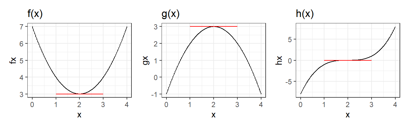 

In all three cases, the point \(x^*=2\) satisfies \(f'(x^*)=0\), \(g'(x^*)=0\) and \(h'(x^*)=0\), but in the case of \(h(x)\), \(x^*=2\) is neither a maximum or minimum point (it is an inflection point).

Quite often we find ourselves in situations where our function behaves like \(f(x)\) or \(g(x)\) in the example above, in which case the first order condition does pick out the strict minimum or strict maximum point. For twice-differentiable functions we can use the second-order derivative to see if we are indeed working with such functions. If

  3a.   \(f''(x) > 0\) for all \(x \in (a,b)\)

then the point \(x^*\) such that \(f'(x^*)=0\) gives the minimum point of the function. The condition 3a says that moving from left to right the slope of the function always increases, so the function arcs upwards (we say the function is convex, or convex upwards). If

  3b.   \(f''(x) < 0\) for all \(x \in (a,b)\), then the slope of the function is always decreases as \(x\) increases. The function therefore arcs downwards (i.e., is concave, or concave downwards), and the stationary point then gives a strict maximum point.

We refer to \(f'(x^*)=0\) as the “first-order condition”, and \(f''(x^*)>0\) as the “second-order condition” for a minimum, and \(f''(x^*)<0\) as the second-order condition for a maximum.

Example 2.25 The point \(x=2\) is the minimum point of \(f(x)=(x-2)^2+3\) since \(f'(x)=2(x-2)=0\) at \(x=2\) and \(f''(x)=2>0\) for all \(x\). The point \(x=2\) is the maximum point of \(g(x)=-(x-2)^2-3\) since \(f'(x)=-2(x-2)=0\) at \(x=2\) and \(f''(x)=-2<0\) for all \(x\). The first derivative of the function \(h(x)=(x-2)^3\) is zero at \(x=2\): \(h'(x)=3(x-2)^2=0\) at \(x=2\). However, it fails the second order condition for both a maximum and a minimum as \(h''(x)=6(x-2)\) is neither always positive or always negative.

Note the \(f(x^*)=0\) together with \(f''(x^*)>0\) or \(f''(x^*)<0\) is sufficient to guarantee that \(x^*\) is a minimum or maximum point, but they are not necessary conditions. In \(h(x)\) above, the point \(x=2\) turned out to be neither a maximum or a minimum of the function \(h(x)=(x-2)^3\), but we could not have claimed this solely on the basis of the function’s failure to satisfy the second-order condition. It is possible for a function to fail the second-order condition and yet yield a maximum or minimum point at the point \(x^*\) where the first derivative is zero.

Example 2.26 Suppose we wish to maximize the function \(f(x) = e^{-x^2}\) defined over the open interval \((-\infty,\infty)\). It is twice-differentiable everywhere on this interval. The first derivative is \(f'(x) = -2xe^{-x^2}\) which is zero at \(x=0\) so \(x=0\) is a candidate maximum point. However, the second derivative \[ f''(x)=2e^{-x^2}(2x^2-1) \] is not strictly positive or strictly negative everywhere: \(f''(x)<0\) when \(-1\sqrt{2} < x < 1/\sqrt{2}\), and \(f''(x)>0\) when \(x<-1\sqrt{2}\) or \(x>1\sqrt{2}\). It fails to satisfy the second-order condition for a maximum (or a minimum). Yet the point \(x=0\) is a maximum point (see plot below).

x <- seq(-4,4, by=0.01)
fx <- exp(-x^2)
dat <- data.frame(x=x,fx=fx)
ggplot(data=dat) + geom_line(aes(x=x,y=fx)) + ggtitle("f(x)") +
      geom_segment(aes(x=-1,y=1,xend=1,yend=1), color='red') +
      theme(plot.title = element_text(size = 10)) + theme_bw()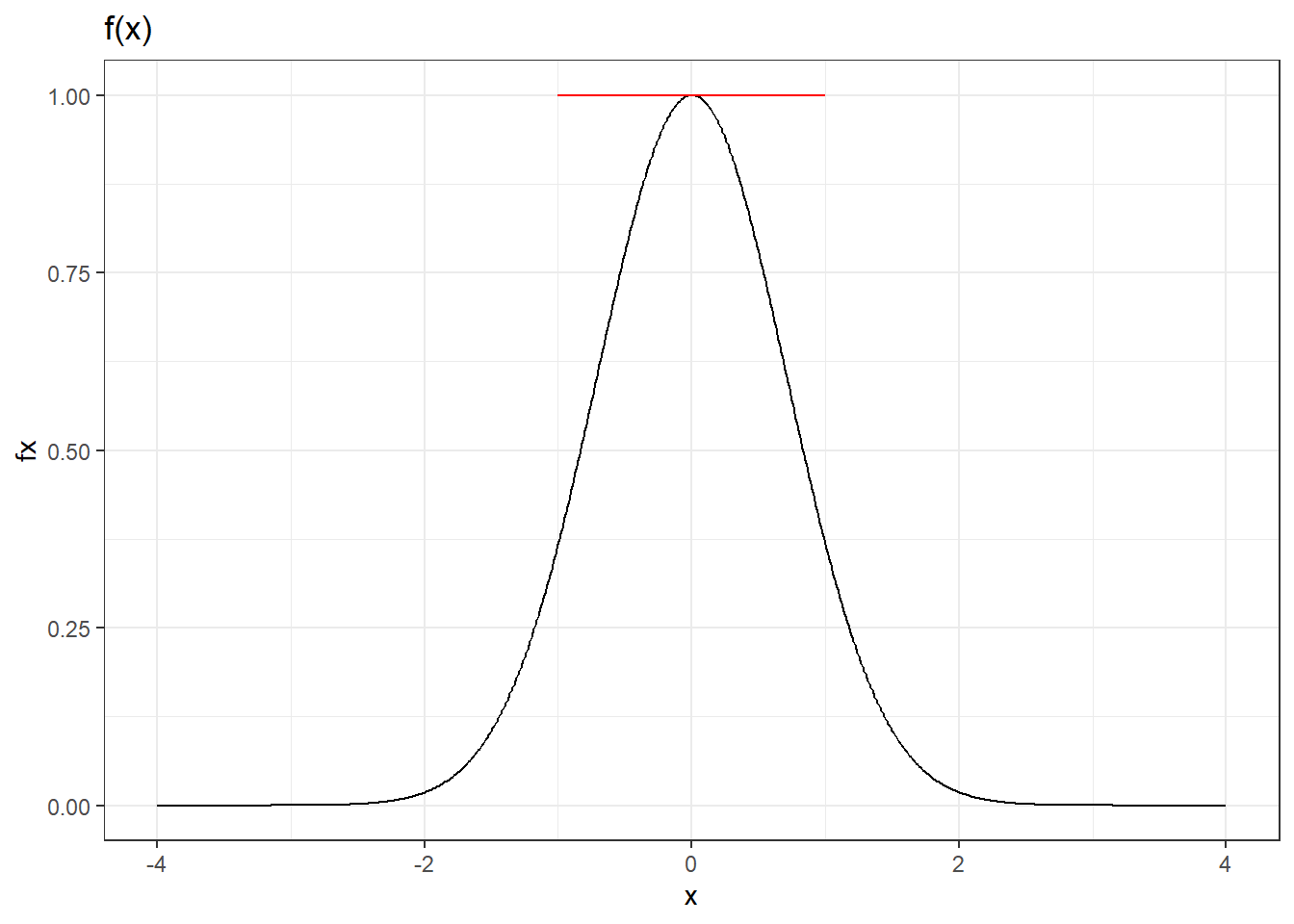

We have noted that the first order condition (2.8) cannot distinguish between maximum and minimum points. It also cannot distinguish between strict vs non-strict maximum/minimum points.

Example 2.27 Consider the function \(f(x) = x^2\exp(-x^2)\) shown below.

x <- seq(-3,3, by=0.01)
f <- function(x){x^2*exp(-x^2)}
dat <- data.frame(x=x,fx=f(x))
x1 <- -1; x2 <- 0; x3 <- 1 
ggplot(data=dat) + geom_line(aes(x=x,y=fx)) + 
      ggtitle("f(x)=x^2*exp(-x/2)") + ylab("") +
      geom_segment(aes(x=x1-0.25,y=f(x1),xend=x1+0.25,yend=f(x1)), color='red') +
      geom_segment(aes(x=x2-0.25,y=0,xend=x2+0.25,yend=0), color='red') +      
      geom_segment(aes(x=x3-0.25,y=f(x3),xend=x3+0.25,yend=f(x3)), color='red') +
      theme(plot.title = element_text(size = 9)) + theme_bw()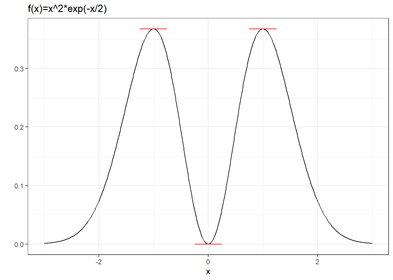

This function has three stationary points. The points \(x=-1\) and \(x=1\) are (non-strict) maximum points. The point \(x=0\) is a strict minimum point.

We have shown an example where the first order condition yields neither a maximum point nor minimum point. Sometimes the first order condition yields points that are maximum or minimum, but only “locally” so.

Example 2.28 Take the function \(f(x) = (x-0.5)^2\exp(-x^2)\) shown below.

x <- seq(-3,3, by=0.01)
f <- function(x){(x-0.5)^2*exp(-x^2)}
dat <- data.frame(x=x,fx=f(x))
x1 <- (1-sqrt(17))/4; x2 <- 0.5; x3 <- (1+sqrt(17))/4 
ggplot(data=dat) + geom_line(aes(x=x,y=fx)) + ggtitle("f(x)") + ylab("") +
      geom_segment(aes(x=x1-0.25,y=f(x1),xend=x1+0.25,yend=f(x1)), color='red') +
      geom_segment(aes(x=x2-0.25,y=0,xend=x2+0.15,yend=0), color='red') +      
      geom_segment(aes(x=x3-0.25,y=f(x3),xend=x3+0.25,yend=f(x3)), color='red') +
      theme(plot.title = element_text(size = 9))  + theme_bw()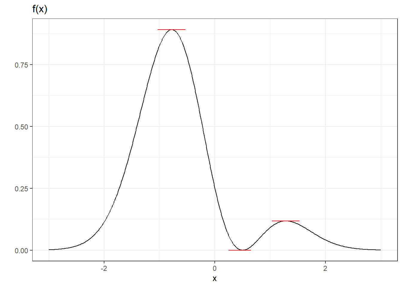

In this example the first order condition picks out three candidate maximum and minimum points. The points \(x=(1-\sqrt{17})/4 \approx -0.78\) is a strict maximum point, where as \(x=0.5\) is a strict minimum point. The point \(x=(1+\sqrt{17})/4 \approx 1.28\) is strictly speaking not a maximum point, but it is if we consider only a small enough neighborhood about \(x=(1+\sqrt{17})/4\). We call this a local maximum point. The first order condition picks out local maximum and local minimum points, in addition to the “global” ones.

Concave/convex functions need not have maximum/minimum points.

Example 2.29 Let \(f(x)=1-1/x\), \(x \in (0,\infty)\). This function is twice-differentiable over its domain which is an open interval. We have \(f'(x)=1/x^2\) and \(f''(x)=-2/x^3\). The second derivative is negative for all \(x \in (0,\infty)\). However, there is no point \(x^*\) such that \(f'(x^*)=0\). The function is concave, but it is strictly increasing and has no maximum point (even though it is bounded from above!).

The discussion above assume twice-differentiable functions defined over open intervals. Things can get a little more complicated once we depart from this scenario, as the following examples show:

Example 2.30 The function \(f(x)=|x|\) has a minimum point at \(x=0\). Yet there are no points at which \(f'(x)=0\) (the function is not differentiable at \(x=0\)).

Example 2.31 Consider the function \(f(x)=x^2\) defined over the restricted domain \(x \in [1,2]\). Note that the domain is now not an open interval. At no point in the domain do we have \(f'(x)=0\). Yet \(x=2\) is a global maximum point, and \(x=1\) is a global minimum point.

For the moment, we will not need to go beyond the class of twice-differentiable concave/convex functions defined over an open interval. However, we will have to consider functions of many variables.

2.3.2 Functions of Many Variables

We will only consider the simplest cases. First consider a function \(f(x,y)\), and assume that the first and second partial derivatives exist everywhere in its domain, which we take to be \(\mathbb{R}^2\). The first order condition in this case is that a minimum or maximum point \((x^*,y^*)\), if it exists, must satisfy \[ \begin{aligned} f_x'(x^*,y^*) &= 0 \\ f_y'(x^*,y^*) &= 0 \end{aligned} \tag{2.9}\] Intuitively, if the slope of the function at \((x^*,y^*)\) in any given direction is not zero, then we can increase or decrease the function by moving along that direction. If (2.9) holds, then the slope of the function in the \(x\)-direction and the \(y\)-direction are both zero at the stationary point \((x^*,y^*)\). This in turn guarantees that the slope in every direction is zero.

Like the univariate case, (2.9) is only necessary, not sufficient. The plots below are three-dimensional plots, from left to right, of the functions \[ f(x,y)=x^2+y^2\;,\; f(x,y)=-x^2-y^2 \;\; \text{and} \;\; f(x,y)=x^2-y^2 \;. \]

x <- y <- seq(-10,10,length.out=30)
funcs <- list(NA,NA,NA)
funcs[[1]] <- function(x,y){r <- x^2 + y^2}
funcs[[2]] <- function(x,y){r <- -x^2 - y^2}
funcs[[3]] <- function(x,y){r <- x^2 - y^2}
fneqs<-c("x^2+y^2","-x^2-y^2","x^2-y^2")
op <- par(bg="white", oma=c(0,0,0,0), mfrow=c(1,3))
for (i in 1:3){
  z <- outer(x,y,funcs[[i]])
  z[is.na(z)] <- 1
  par(mar=c(0,2,0,2), pin=c(2,2.5))
  persp(x,y,z,theta=30, phi=10,r=10, expand=0.8, col="cadetblue1",
      ltheta=120, shade=0.75,ticktype="detailed", xlab="X", ylab="Y", zlab="")
  mtext(fneqs[i],side=3, line=-3, adj=0)
}
mtext("Three functions with stationary point at (0,0)", line=-3, side=1, outer=TRUE)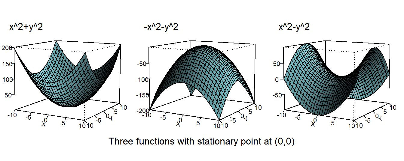

All three have a stationary point at \((x^*,y^*)=(0,0)\), but in the first case we have a minimum, in the second a maximum, and in the third case neither. In the first case, the function is convex throughout. In the second, the function is concave throughout, and in the third case neither. For the most part we will deal with concave or convex functions. How do we tell if a function is concave or convex? For functions of one variable we look at the second derivative. For a function of many variables, we look at the matrix of second-order partial derivatives. For example, for the function \(f(x,y,z)\), we would look at the matrix \[ H_f = \begin{bmatrix} \dfrac{\partial^2 f}{\partial x^2} & \dfrac{\partial^2 f}{\partial x \partial y} & \dfrac{\partial^2 f}{\partial x \partial z} \\ \dfrac{\partial^2 f}{\partial y \partial x} & \dfrac{\partial^2 f}{\partial y^2} & \dfrac{\partial^2 f}{\partial y \partial z} \\ \dfrac{\partial^2 f}{\partial z \partial x} & \dfrac{\partial^2 f}{\partial z \partial y} & \dfrac{\partial^2 f}{\partial z^2} \end{bmatrix} \] This matrix, which is symmetric, is called the Hessian of the function \(f\). If it is the case that the Hessian satisfies \[ a'H_fa > 0 \tag{2.10}\] for all non-zero vectors \(a\), then the function is convex (we also say that the Hessian is positive definite). In this case we say that the “second-order condition” for a minimum holds, and the stationary point is a minimum point. If \[ a'H_fa < 0 \tag{2.11}\] then the Hessian is negative definitive, and the function is concave. The second-order condition for a maximum holds, and the stationary point is the maximum point. If neither condition holds, then the second order condition is silent about the status of the stationary point.

Example 2.32 For the function \(f(x,y)=x^2+y^2\), we have \[ H_f = \begin{bmatrix} \dfrac{\partial^2 f}{\partial x^2} & \dfrac{\partial^2 f}{\partial x \partial y} \\ \dfrac{\partial^2 f}{\partial y \partial x} & \dfrac{\partial^2 f}{\partial y^2} \end{bmatrix} = \begin{bmatrix} 2 & 0 \\ 0 & 2 \end{bmatrix}. \] Therefore \[ a'H_fa = \begin{bmatrix} a_1 & a_2 \end{bmatrix} \begin{bmatrix} 2 & 0 \\ 0 & 2 \end{bmatrix} \begin{bmatrix} a_1 \\ a_2 \end{bmatrix} = 2a_1^2+2a_2^2 \] which is strictly positive for all non-zero vectors \(a\).

For the function \(f(x,y)=-x^2-y^2\), we have \[ a'H_fa = \begin{bmatrix} a_1 & a_2 \end{bmatrix} \begin{bmatrix} -2 & 0 \\ 0 & -2 \end{bmatrix} \begin{bmatrix} a_1 \\ a_2 \end{bmatrix} = -2(a_1^2+a_2^2) \] which is strictly negative for all non-zero vectors \(a\). In the case of \(f(x,y)=x^2-y^2\), we have \[ a'H_fa = \begin{bmatrix} a_1 & a_2 \end{bmatrix} \begin{bmatrix} 2 & 0 \\ 0 & -2 \end{bmatrix} \begin{bmatrix} a_1 \\ a_2 \end{bmatrix} = 2(a_1^2-a_2^2) \] which can be negative or positive or zero, depending on the values of \(a_1\) and \(a_2\).

The first and second order conditions stated in this section extend to functions of more than two variables.

2.3.3 Exercises

Exercise 2.32 Find the first and second derivatives of the function \[ f(x)=\dfrac{x}{1+x^2}\,. \] Show that \(f'(x)=0\) at \(x=1\) and \(x=-1\). Find the regions over which \(f''(x)\) is positive, and the regions over which \(f''(x)\) is negative. What argument can you give to prove that \(x=1\) is a global maximum point, and \(x=-1\) is a global minimum point of the function?

Exercise 2.33 Let \(\{X_i\}_{i=1}^N\) be a sample of \(N\) observations of a random variable \(X\) with population mean \(\mathrm{E}[X]=\mu\). Show that the sample mean \(\hat{\mu} = \frac{1}{N}\sum_{i=1}^N X_i\) minimizes the function \[ f(\hat{\mu}) = \sum_{i=1}^N (X_i-\hat{\mu})^2. \]

Exercise 2.34 Show that \(f(x)=2x^3 - 6x\) has stationary points at \(x=1\) and \(x=-1\). Show that \(x=-1\) is a local maximum point, and \(x=1\) is a local minimum point.

Exercise 2.35 Let \(A\) be the following matrix, which can be decomposed into the product of two matrices as shown: \[ A = \begin{bmatrix} 5 & 5 \\ 5 & 10 \end{bmatrix} = \begin{bmatrix} 1 & 2 \\ 3 & 1 \end{bmatrix} \begin{bmatrix} 1 & 3 \\ 2 & 1 \end{bmatrix} \;. \] Explain why this shows \(A\) is positive definite. Find the stationary point of the function \[ f(x,y)=5x^2 + 10xy + 10y^2. \] Is this point a maximum point, a minimum point, or neither?

2.4 Application: Fitting a Straight Line by Least Squares

For an application of the ideas we have just reviewed, consider the problem of fitting a straight line through a scatterplot of \(n\) points \(\{X_{i},Y_{i}\}_{i=1}^{n}\). For illustration, we will use data in the file ols01.csv which comprises 10 observations of variables \(X\) and \(Y\).

# The function read_csv() is from tidyverse::readr
# The option show_col_types=F shuts some automated messages from read_csv()
df <- read_csv("data\\ols01.csv", show_col_types=F)
glimpse(df)     # tidyverse version of str() to quickly explore tibble

Rows: 10
Columns: 2
$ X <dbl> 2.514333, 5.169248, 1.731986, 3.421461, 4.028095, 4.577327, 8.194569…
$ Y <dbl> 7.639444, 10.668647, 3.110330, 1.846599, 11.782167, 10.582858, 15.45…

The glimpse() function gives you a quick look at the data. Although the data is presented in transposed form, there are 2 columns of data, 10 rows each. The data are plotted in Fig. 2.1.

p1 <- df %>%  
  ggplot(aes(x=X,y=Y)) + geom_point(size=1) + theme_minimal() + 
  xlim(0,10) + ylim(0,16) + coord_fixed(ratio=1/3) + 
  theme(axis.title=element_text(size=10))
p1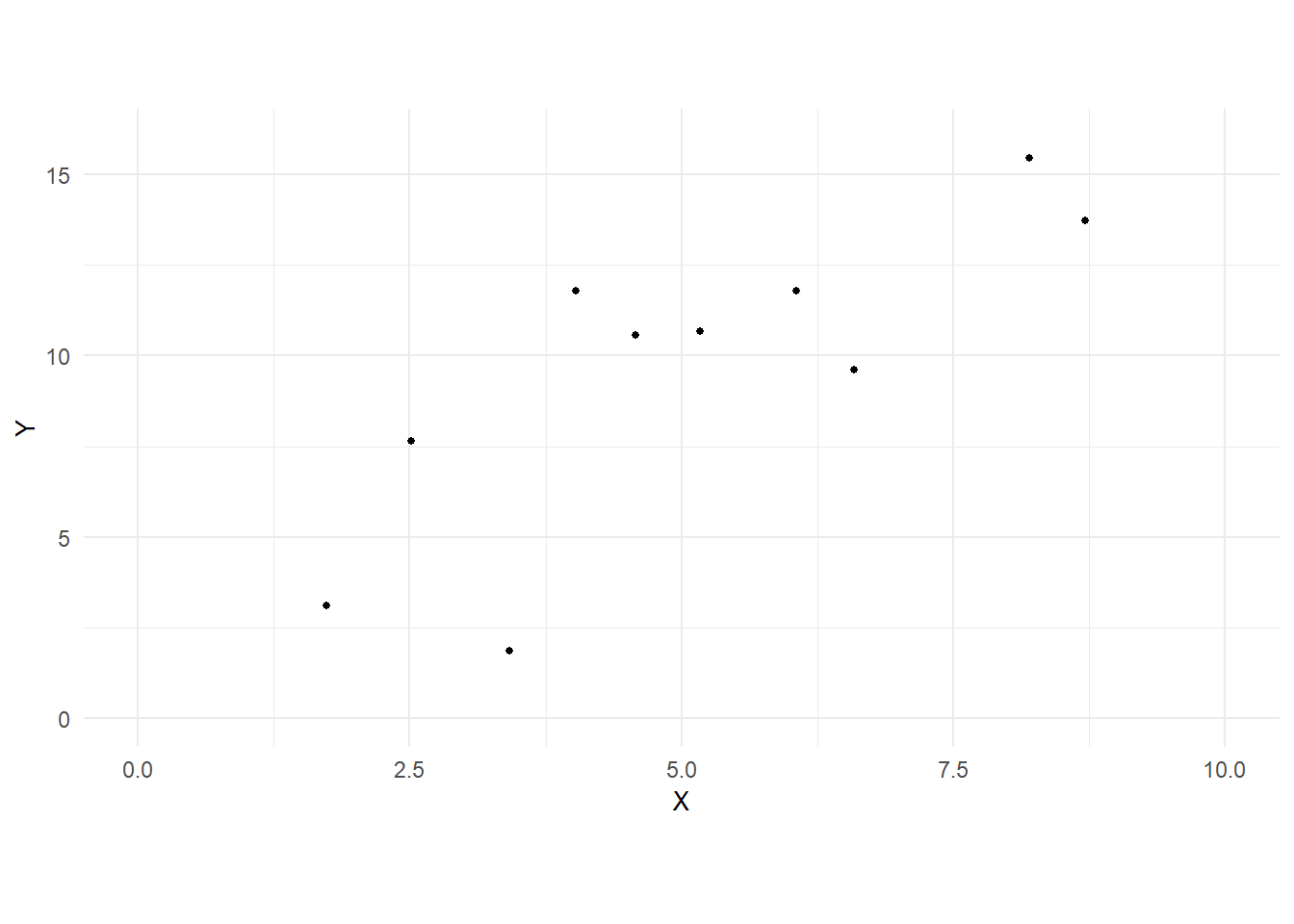

Figure 2.1: The data set ols01.csv.

There are many ways to fit a straight line through these points, including

1. minimizing the sum of vertical distances from each point to the line;
2. minimizing the sum of horizontal distances from each point to the line;
3. minimizing the sum perpendicular distances from each point to the line;
4. use the square distances rather than the absolute distances;
5. give different weights to each observation.

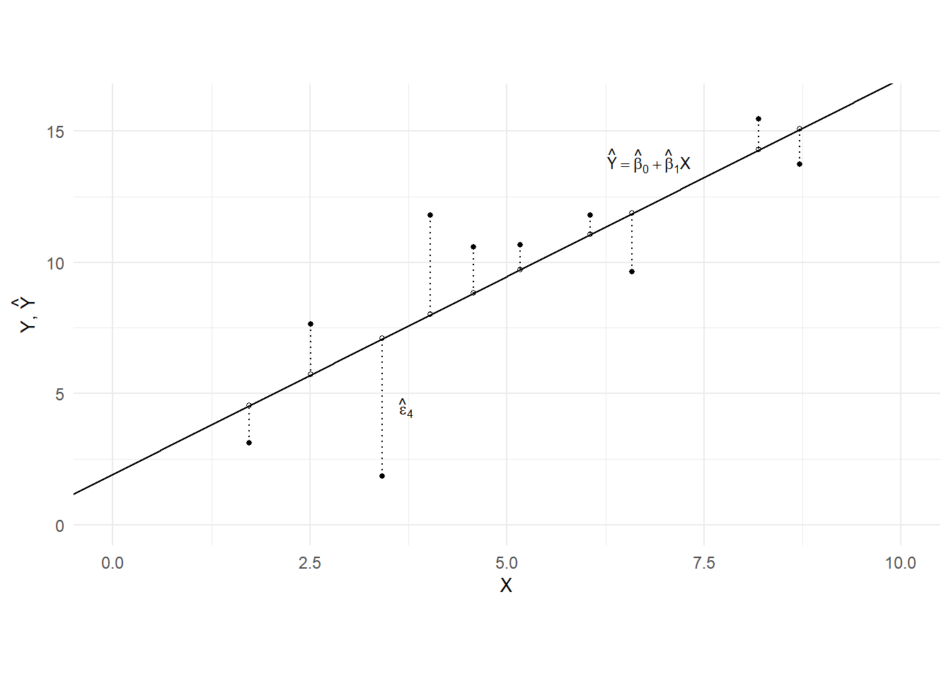
You can think of many other variations. For this exercise, we will minimize the sum of the squared vertical distances of each observation to the fitted line (we will refer to this as “ordinary least squares” or “OLS”). The vertical distances are marked out in Fig. 2.2. For the moment there is no particular reason for choosing this method, and no statistical / probabilistic / econometric meaning to this exercise at all. We are simply fitting a straight line to the data points, and exploring the mathematical properties of such a line. Everything we say in this section will apply to any set of data points \(\{X_{i},Y_{i}\}_{i=1}^{n}\), regardless of the source of the data.

Write the line to be fitted as \[ \hat{Y} = \hat{\beta}_{0} + \hat{\beta}_{1} X \] where \(\hat{\beta}_{0}\) and \(\hat{\beta}_{1}\) are the \(y\)-intercept and slope of the line respectively. Choosing a straight line means choosing values for these two objects. For each \(i=1,2,...,n\), let \(\hat{Y}_{i}\) be the \(y\)-value of this line at \(X = X_{i}\) (the points \((X_{i},\hat{Y}_{i})\) are shown on Fig. 2.2 as hollow circles). Then the vertical distances from the data points to the line, are \(Y_{i}-\hat{Y}_{i}\) which we will denote by \(\hat{\epsilon}_{i}\): \[ \hat{\epsilon}_{i} = Y_{i} - \hat{Y}_{i} \quad \text{where} \quad \hat{Y}_{i} = \hat{\beta}_{0} + \hat{\beta}_{1}X_{i}\;. \] We will call \(\hat{Y}_{i}\) the “fitted values” of \(Y\), and \(\hat{\epsilon}_{i}\) the “residuals”. The residual for the fourth observation in our data set is marked out in Fig. 2.2. ¹

Figure 2.2: Fitting a Straight Line to Data by Least Squares.

The sum of squared vertical distances, or “sum of squared residuals” can then be written as \[ SSR = \sum_{i=1}^N \hat{\epsilon_i}^2 = \sum_{i=1}^N (Y_i - \hat{\beta}_0 - \hat{\beta}_1X_i)^2. \tag{2.12}\]

We want to

• derive the formulas for \(\hat{\beta}_{0}\) and \(\hat{\beta}_{1}\) that minimizes the expression in (5.5).
• understand the algebraic properties of OLS estimators.

Once again, we are not making any statistical or econometric interpretations at this point.

Let \(\hat{\beta}_0^{ols}\) and \(\hat{\beta}_1^{ols}\) be the values of \(\hat{\beta}_0\) and \(\hat{\beta}_1\) that minimizes SSR in (5.5). These can be found by solving the first order conditions: \[ \begin{aligned} \left.\frac{\partial SSR}{\partial \hat{\beta}_0}\right| _{\hat{\beta}_0^{ols},\,\hat{\beta}_1^{ols}} &= -2\sum_{i=1}^N(Y_i-\hat{\beta}_0^{ols}-\hat{\beta}_1^{ols}X_i)=0 \\ \left.\frac{\partial SSR}{\partial \hat{\beta}_1}\right| _{\hat{\beta}_0^{ols},\,\hat{\beta}_1^{ols}} &= -2\sum_{i=1}^N(Y_i-\hat{\beta}_0^{ols}-\hat{\beta}_1^{ols}X_i)X_i=0 \end{aligned} \tag{2.13}\] where the notation \(\left.\frac{\partial SSR}{\partial \hat{\beta}_0}\right|_{\hat{\beta}_0^{ols},\,\hat{\beta}_1^{ols}}\) refers to the derivative \(\frac{\partial SSR}{\partial \hat{\beta}_0}\) evaluated at \(\hat{\beta}_0^{ols}\) and \(\hat{\beta}_1^{ols}\), and likewise for \(\left.\frac{\partial SSR}{\partial \hat{\beta}_1}\right|_{\hat{\beta}_0^{ols},\,\hat{\beta}_1^{ols}}\).

We can solve the equations in (2.13) in the following way. Divide the first equation in (2.13) by \(N\) and solve for \(\hat{\beta}_0^{ols}\) to get \[ \hat{\beta}_0^{ols} = \overline{Y} - \hat{\beta}_1^{ols}\overline{X}\,. \tag{2.14}\] Then substitute (2.14) into the second equation. This gives \[ \sum_{i=1}^N ( (Y_i-\overline{Y}) - \hat{\beta}_1^{ols}(X_i-\overline{X}))X_i =0 \] which we can solve to get \[ \hat{\beta}_1^{ols} = \frac{\sum_{i=1}^N (Y_i-\overline{Y})X_i}{\sum_{i=1}^N(X_i-\overline{X})X_i}\,. \tag{2.15}\] We can substitute this expression back into (2.14) to get the full formula for \(\hat{\beta}_{0}^{ols}\), but we’ll leave (2.14) as it is.

We can show that the second order condition for a global minimum is satisfied, so that \(\hat{\beta}_{0}^{ols}\) and \(\hat{\beta}_{1}^{ols}\) does in fact minimize the SSR. This is left as an exercise.

The fitted line is therefore \[ \hat{Y} = \hat{\beta}_{0}^{ols} + \hat{\beta}_{1}^{ols} X \] where \(\hat{\beta}_{0}^{ols}\) and \(\hat{\beta}_{1}^{ols}\) are as given in (2.14) and (2.15). For our data, we have

beta1hat = sum((df$X - mean(df$X)) * df$Y) / sum((df$X - mean(df$X))^2)  
beta0hat = mean(df$Y) - beta1hat*mean(df$X)
cat("Intercept:", round(beta0hat,3), "; Slope:", round(beta1hat,3))

Intercept: 1.943 ; Slope: 1.506

2.4.1 Algebraic Properties

From this point on, we will refer to the fitted line as the “sample regression line”. The fitted values \(\hat{Y}_{i}\) and residuals \(\hat{\epsilon}_{i}\) should be understood to be the “least squares” or “OLS” fitted values and residuals, i.e., \[ \hat{Y}_{i} = \hat{\beta}_{0}^{ols} + \hat{\beta}_{1}^{ols} X_{i} \quad \text{and} \quad \hat{\epsilon}_{i} = Y_{i} - \hat{Y}_{i} = Y_{i} - \hat{\beta}_{0}^{ols} - \hat{\beta}_{1}^{ols} X_{i}\,. \] Ideally we ought to place “\(ols\)” superscripts on these, to distinguish them from fitted values and residuals obtained from other fitting methods, but we will neglect this detail. We will leave the superscripts on \(\hat{\beta}_{0}^{ols}\) and \(\hat{\beta}_{1}^{ols}\). We call \(\{Y_{i}\}\) the regressand, and \(\{X_{i}\}\) the regressor.

The sample regression line has a number of useful algebraic properties.

If all of the \(X\) observations are of the same value, i.e., \(X_{1}=X_{2}= ...=X_{N}\), then \(\overline{X}\) will have this same value, and \({\sum_{i=1}^N(X_i-\overline{X})X_i}\) will be zero. As a result, we will not be able to compute (2.15) (nor (2.14). This is the case where all of your data points line up in a vertical straight line.

Since
\[ \sum_{i=1}^N (X_i-\overline{X})(Y_i-\overline{Y}) = \sum_{i=1}^N (X_i-\overline{X})Y_i \quad \text{and} \quad \sum_{i=1}^N (X_i-\overline{X})^2 = \sum_{i=1}^N (X_i-\overline{X})X_i \,, \] we can write (2.15) as \[ \hat{\beta}_1^{ols} \;=\; \frac{\sum_{i=1}^N (X_i-\overline{X})Y_i}{\sum_{i=1}^N(X_i-\overline{X})X_i} \;=\; \frac{\sum_{i=1}^N (X_i-\overline{X})(Y_i-\overline{Y})}{\sum_{i=1}^N(X_i-\overline{X})^2}\;. \tag{2.16}\] If you divide both numerator and denominator by \(N-1\), the numerator becomes the sample covariance of \(X_{i}\) and \(Y_{i}\), and the denominator becomes the sample variance of \(X_{i}\).

The first equation in the first order condition (2.13) can be written as \[ \sum_{i=1}^N(Y_i-\hat{\beta}_0^{ols}-\hat{\beta}_1^{ols}X_i) = \sum_{i=1}^N \hat{\epsilon}_{i} = 0\,. \tag{2.17}\] It follows that the sample mean of the least squares residuals is zero.

The second equation in the first order condition (2.13) can be written as \[ \sum_{i=1}^N(Y_i-\hat{\beta}_0^{ols}-\hat{\beta}_1^{ols}X_i)X_{i} = \sum_{i=1}^N \hat{\epsilon}_{i}X_{i} = 0\,. \tag{2.18}\] We say that the OLS residuals \(\hat{\epsilon}_{i}\) and the regressors \(X_{i}\) are orthogonal. This result and [P3] imply that the fitted values and the residuals are also orthogonal. \[ \sum_{i=1}^N \hat{Y}_i \hat{\epsilon}_{i} = \hat{\beta}_0^{ols}\sum_{i=1}^N \hat{\epsilon}_{i} + \hat{\beta}_1^{ols}\sum_{i=1}^N X_{i}\hat{\epsilon}_{i} = 0\,. \tag{2.19}\]

Because the residuals have sample mean zero, it follows from (2.18) that the sample covariance between the residuals and the regressors is zero. This is because the sample covariance is \(\frac{1}{N}\sum_{i=1}^N (\hat{\epsilon}_{i} - \overline{\epsilon}_{i})(X_{i}-\overline{X})\) and \[ \begin{aligned} \sum_{i=1}^N (\hat{\epsilon}_{i} - \overline{\epsilon}_{i})(X_{i}-\overline{X}) &= \sum_{i=1}^N (\hat{\epsilon}_{i} - \overline{\epsilon}_{i})X_{i} \qquad \text{(why?)} \\ &= \sum_{i=1}^N \hat{\epsilon}_{i}X_{i} \qquad \text{(why?)} \\ \end{aligned} \] Summing the equation \[ Y_{i} = \hat{\beta}_{0}^{ols} + \hat{\beta}_{1}^{ols} X_{i} + \hat{\epsilon}_{i} \] over \(i=1,2,...,N\) and dividing by \(N\) gives \[ \overline{Y} =\, \hat{\beta}_{0}^{ols} + \hat{\beta}_{1}^{ols} \overline{X} \] since the residuals have sample mean zero. This means that the sample regression line (the fitted line) passes through the point \((\overline{X}, \overline{Y})\).

Similarly, taking sample means on both sides of \(Y_{i} = \hat{Y}_{i} + \hat{\epsilon}_{i}\) gives \[ \overline{Y} = \overline{\hat{Y}}\,, \qquad \text{where}\;\; \overline{\hat{Y}} = (1/N) \sum_{i=1}^{N} \hat{Y}_{i}\,. \] In words, the OLS fitted values and the regressand both have the same sample mean.

We have the useful decomposition \[ \sum_{i=1}^N (Y_i - \overline{Y})^2 = \sum_{i=1}^N (\hat{Y}_i - \overline{\hat{Y}})^2 + \sum_{i=1}^N \hat{\epsilon}_i^2. \tag{2.20}\] We read (2.20) as “Sum of Squared Total = Sum of Squared Explained + Sum of Squared Residuals” or “SST = SSE + SSR”. It is essentially a variance decomposition result. To get this result, substract \(\overline{Y}\) on both sides, then square and sum both sides: \[ \begin{gathered} Y_i = \hat{Y}_i + \hat{\epsilon}_i \\ Y_i - \overline{Y} = \hat{Y}_i - \overline{Y}+ \hat{\epsilon}_i \\ (Y_i - \overline{Y})^2 = (\hat{Y}_i - \overline{Y})^2 + \hat{\epsilon}_i^2 + 2(\hat{Y}_i - \overline{Y})\hat{\epsilon}_i \\ \sum_{i=1}^N(Y_i - \overline{Y})^2 = \sum_{i=1}^N(\hat{Y}_i - \overline{Y})^2 + \sum_{i=1}^N\hat{\epsilon}_i^2 + 2\sum_{i=1}^N(\hat{Y}_i - \overline{Y})\hat{\epsilon}_i\;. \end{gathered} \] Since \(\overline{Y}=\overline{\hat{Y}}\), replace \(\sum_{i=1}^N(\hat{Y}_i - \overline{Y})^2\) with \(\sum_{i=1}^N(\hat{Y}_i - \overline{\hat{Y}})^2\). Complete the proof by noting that \[ \sum_{i=1}^N(\hat{Y}_i - \overline{Y})\hat{\epsilon}_i = \sum_{i=1}^N \hat{Y}_i\hat{\epsilon}_i - \overline{Y}\sum_{i=1}^N\hat{\epsilon}_i = 0\,. \]

The identity in (2.20) forms the basis of the classic “goodness-of-fit” \(R^2\) measure. We can think of the SST as a measure of the total “variation” in \(Y_{i}\). Dividing by \(N-1\) gives you the sample variance of \(Y_{i}\). The SST is decomposed into the total “variation in \(\hat{Y}_{i}\) and the residuals. Dividing (2.20) throughout by SST, we have \[ 1 = \frac{SSE}{SST} + \frac{SSR}{SST} \] from which we can define \[ R^2 = 1 - \frac{SSR}{SST}\;. \tag{2.21}\]

Since \(1-SSR/SST = SSE/SST\), the \(R^2\) has the interpretation as the proportion of variation in \(Y_i\) that is accounted for (sometimes the word “explained” is used) by \(\hat{Y}_i\), or by \(X_{i}\), since \(\hat{Y}_{i}\) is just a linear function of \(X_{i}\).

By construction, \(R^2\) lies between 0 and 1 (inclusive). An \(R^2\) of one indicates a perfect fit, since \(R^2=1\) only when \(SSR=0\), which means that \(\hat{\epsilon}_i=0\) for all \(i\). On the other hand, \(R^2 = 0\) when \(SSR=SST\), which means that \(SSE=\sum_{i=1}^N (\hat{Y}_i - \overline{Y})^2=0\), or \(\hat{Y}_i = \overline{Y}\) for all \(i\) (this implies also that \(\hat{\beta}_1=0\)). All intermediate fits result in values of \(R^2\) strictly between 0 and 1.

For our data set and regression, we have

ehat <- df$Y - Yhat
SSR <- sum(ehat^2)  # we defined ehat = residuals(mdl) earlier
SST <- sum((df$Y-mean(df$Y))^2)
Rsqr <- 1 - SSR/SST
print(paste("The R-squared for the sample regression line is:", round(Rsqr,3)))

[1] "The R-squared for the sample regression line is: 0.644"

That is, the fitted line accounts for around 64.5 percent of the variation in \(Y_{i}\).

As you might have guessed, there are built-in function in R for making all the computations demonstrated here. The usual function for calculating the coefficient values is lm() from the (auto-loaded) package stats.

  mdl <- lm(Y~X, data=df)  # Y~X means regress Y on X, including an intercept term.
  coef(mdl) # "mdl" contains a lot of stuff, coef(mdl) picks out the coefficient vector.

(Intercept)           X 
   1.943349    1.506138 

We can get the fitted values and residuals using

  Yhat <- fitted(mdl)
  ehat <- residuals(mdl)

We can extract the \(R^2\) from the summary.lm object returned when summary() function is applied to the lm object mdl:

summary(mdl)$r.squared

[1] 0.6444797

2.5 Exercises

Exercise 2.36 Show that \(\hat{\beta}_{1}^{ols}\) in (2.15) can be written as \(\hat{\beta}_{1}^{ols} = \frac{\sum_{i=1}^NX_iY_i - N\overline{X}\,\overline{Y}} {\sum_{i=1}^NX_i^2 - N\overline{X}^2}\).

Exercise 2.37 The second order condition for the OLS minimization of the SSR in (5.5) is that \[ H = \begin{bmatrix} \dfrac{\partial^2SSR}{\partial\hat{\beta}_0^2} & \dfrac{\partial^2SSR}{\partial\hat{\beta}_0\partial\hat{\beta}_1} \\ \dfrac{\partial^2SSR}{\partial\hat{\beta}_0\partial\hat{\beta}_1} & \dfrac{\partial^2SSR}{\partial\hat{\beta}_1^2} \end{bmatrix} \; \text{ is positive definite.} \] i.e., \(c^\mathrm{T}Hc > 0\) for all \(c \neq 0\). Show that this condition is satisfied. Hint: Show that \[ H = 2 \begin{bmatrix} N & \sum_{i=1}^N X_i \\ \sum_{i=1}^N X_i & \sum_{i=1}^N X_i^2 \end{bmatrix} = 2(X^\mathrm{T}X) \quad \text{where} \quad X = \begin{bmatrix} 1 & X_1 \\ 1 & X_2 \\ \vdots & \vdots \\ 1 & X_N \end{bmatrix} \] and explain why this implies that \(H\) is positive definite, assuming \(\sum_{i=1}^N (X_i-\overline{X})^2 \neq 0\).

Exercise 2.38 In order to fit the straight line to your data points by least squares, you require the condition that \(\sum_{i=1}^N (X_i - \overline{X})^2 \neq 0\), i.e., \(X_i\) cannot all be equal to a single constant value. What is \(\hat{\beta}_{0}^{ols}\) and \(\hat{\beta}_{1}^{ols}\) if this condition is met, but \(Y_i = c\) for all \(i=1,...,N\)? What is the \(R^2\) in this case?

Exercise 2.39 Suppose you fit a straight line to your data with the additional constraint that the line must pass through the origin. In other words, you fit the sample regression line \[ \hat{Y}_{i} = \hat{\beta}_{1} X_{i} \] to your data points. Find the value of \(\hat{\beta}_{1}\) that minimizes the sum of squared residuals, where the residuals are now \(\hat{\epsilon}_{i} = Y_{i} - \hat{\beta}_{1} X_{i}\).

Which algebraic properties of the sample regression line [P1]-[P8] continue to hold and which are lost? Will the \(R^2\) as defined in (2.21) still necessarily lie between 0 and 1? (Hint: it can go below 0, but why?) What does it mean if it goes below zero?

Exercise 2.40 (Continuing with the straight line passing through the origin.) The formula for \(\hat{\beta}_1\) when fitting the straight line with no intercept \(\hat{Y} = \hat{\beta}_1 X\) is \[ \hat{\beta}_{1}^{ols} = \frac{\sum_{i=1}^N X_iY_i}{\sum_{i=1}^N X_i^2}\,. \] For this formula to be feasible, we require \(\sum_{i=1}^N X_i^2 \neq 0\), but OLS estimation is still feasible if \(\sum_{i=1}^N (X_i-\overline{X})^2 = 0\). In other words, we no longer require variation in the \(X_{i}\). Why is this so?

International Monetary Fund, International Labour Organization, Statistical Office of the European Union (Eurostat), United Nations Economic Commission for Europe, Organisation for Economic Co-operation and Development (OECD), and The World Bank. 2020. Consumer Price Index Manual: Concepts and Methods 2020. Washington, D.C.: International Monetary Fund.

---

1. I’ll show code for most of the figures in this book, but I’ll skip the code for this figure as it is a bit distracting.