library(tidyverse)
library(patchwork)
library(readxl)
library(sandwich)7 Heteroskedasticity and Specification Tests
We now deal with situations where the conditional variance of the noise term depends on the regressors, i.e., where we have conditional heteroskedasticity. We have already seen that this will not cause bias or inconsistency; we know this because the proofs of unbiasedness and consistency do not make use of the constant conditional variance assumption. However, the derivations of the formulas for the OLS estimator variances and the proof of efficiency of OLS estimators do make use of the constant conditional variance assumption, and so these results no longer apply if there is conditional heteroskedasticity. In this chapter, we present an alternative estimation approach that aims to provide more efficient estimators under this situation. We also present a way of estimating the variance of the OLS coefficient estimators that allows for conditional heteroskedasticity. Finally, we discuss tests for heteroskedasticity, specification form, and normality of noise terms.
We use the following packages in this chapter.
7.1 An Example
We begin with a simple illustrative example where we can directly show all of the consequences of heteroskedasticity.
Example 7.1 Suppose \[ Y_i = \beta_1 X_{i} + \epsilon_i \, , \, i=1,2,...,N \tag{7.1}\] such that \[ \mathrm{E}[\epsilon_{i} | \mathrm{x}] = 0\,,\quad \mathrm{E}[\epsilon_{i}^2 | \mathrm{x}] = \sigma^2X_i^2\,,\quad\text{and}\quad \mathrm{E}[\epsilon_{i}\epsilon_{j} | \mathrm{x}] = 0 \] for all \(i \neq j\), \(i=1,2,...,N\). We also assume that \(\sum_{i=1}^N X_i^2 \neq 0\). (Here \(X_i\) represents the \(i\mathrm{th}\) observation of variable \(X\), and \(\mathrm{x}\) represents all of the observations of \(X_i\).) The OLS estimator for \(\beta_1\) in this example is \[ \hat{\beta}_1^{ols} = \frac{\sum_{i=1}^N X_iY_i}{\sum_{i=1}^N X_i^2} \tag{7.2}\] which is unbiased for \(\beta_1\): writing Eq. 7.2 as \[ \hat{\beta}_1^{ols} = \frac{\sum_{i=1}^N X_iY_i}{\sum_{i=1}^N X_i^2} = \frac{\sum_{i=1}^N X_i(\beta_1 X_i + \epsilon_i)}{\sum_{i=1}^N X_i^2} = \beta_1 + \frac{\sum_{i=1}^N X_i\epsilon_i}{\sum_{i=1}^N X_i^2} \] and taking conditional expectations gives \[ \mathrm{E}[\hat{\beta}_1^{ols}|\mathrm{x}] = \beta_1 + \frac{\sum_{i=1}^N X_i\mathrm{E}[\epsilon_i|\mathrm{x}]}{\sum_{i=1}^N X_i^2} = \beta_1. \] Under our assumptions, the variance of the OLS estimator is \[ \begin{aligned} \mathrm{var}[\hat{\beta}_1^{ols}|\mathrm{x}] &= \frac{\sum_{i=1}^N X_i^2\mathrm{var}[\epsilon_i|\mathrm{x}]}{\left(\sum_{i=1}^N X_i^2\right)^2} \\ &= \frac{\sum_{i=1}^N X_i^2(\sigma^2 X_i^2)}{\left(\sum_{i=1}^N X_i^2\right)^2} = \frac{\sigma^2\sum_{i=1}^N X_i^4}{\left(\sum_{i=1}^N X_i^2\right)^2}\,. \end{aligned} \tag{7.3}\] Had you not realized that there is heteroskedasticity, you would have estimated \(\mathrm{var}[\hat{\beta_1}|\mathrm{x}]\) using the usual OLS formula for the variance when an intercept is excluded, which is \[ \widehat{\mathrm{var}}[\hat{\beta}_1^{ols}|\mathrm{x}] = \frac{s^2}{\sum_{i=1}^N X_i^2} \, , \quad s^2 = \frac{1}{N-1}\sum_{i=1}^N \hat{\epsilon_i}^2 \, , \quad \hat{\epsilon_i} = Y_i - \hat{\beta_1}X_i\, . \] This variance estimator is based on the assumption of conditional homoskedasticity, and is therefore inappropriate for this example. The form is wrong, and it is not immediately clear what \(s^2\) is estimating.
Furthermore, it turns out that the OLS estimator is inefficient. We show this by presenting a more efficient linear unbiased estimator. Weight each observation by \(1/X_i\) and run the regression \[ \frac{Y_i}{X_i} = \beta_1 + \frac{\epsilon_i}{X_i} = \beta_1 + \epsilon_i^*\,. \tag{7.4}\] That is, simply regress \(Y_{i}/X_{i}\) on a constant. The modified noise terms in this regression will continue to have zero conditional expectation \[ \mathrm{E}[\epsilon_i/X_i | \mathrm{x}] = (1/X_i)\mathrm{E}[\epsilon_i | \mathrm{x}] = 0 \] and remain uncorrelated (exercise). Furthermore, its conditional variance is now constant: \[ \mathrm{var}[\epsilon_i/X_i | \mathrm{x}] = (1/X_i^2)\mathrm{var}[\epsilon_i | \mathrm{x}] = \sigma^2\,. \] OLS estimation applied to this modified regression model Eq. 7.4 gives the estimator \[ \hat{\beta}_1^{wls} = \frac{1}{N}\sum_{i=1}^N\frac{Y_i}{X_i} \,. \tag{7.5}\] The ‘wls’ superscript stands for “weighted least squares”. Since Eq. 7.5 can be written as \[ \hat{\beta}_1^{wls} = \sum_{i=1}^N \left( \frac{1}{NX_{i}}\right) Y_i\,, \] it is a linear estimator. Since this estimator arises out a linear regression with homoskedastic and uncorrelated noise terms that have zero conditional expectation, it is unbiased and minimum variance among all linear unbiased estimators.
The fact that \(\hat{\beta}_1^{wls}\) is BLU suggests that \(\hat{\beta}_1^{ols}\) is not. In our simple example, it is straightforward to demonstrate this fact directly. Since \(\hat{\beta}_1^{wls}\) is a sample mean of observations of a random variable with variance \(\sigma^2\), its variance is \[ \mathrm{var}[\hat{\beta}_1^{wls}] = \frac{\sigma^2}{N}\,. \tag{7.6}\] It can be shown (see exercises) that \[ \frac{\sum_{i=1}^N X_i^4}{\left(\sum_{i=1}^N X_i^2\right)^2} \geq \frac{1}{N}\,, \tag{7.7}\] therefore \[ \mathrm{var}[\hat{\beta}_1^{wls}] \leq \mathrm{var}[\hat{\beta}_1^{ols}]\,. \] The reason OLS estimators are inefficient when there is conditional heteroskedasticity is that some observations are less informative about the population regression line than others, but OLS makes no use of this fact. Information ignored leads to inefficiency. The weighted least squares approach, on the other hand, uses this information directly, by assigning less weight to noisier observations, and more weight to observations whose noise terms have lower variance.
We have shown, in the context of a simple example, that the WLS estimator dominates the OLS estimator under conditional heteroskedasticity in the sense that the WLS estimator is (like OLS) linear and unbiased, but more precise. However, to get the WLS estimator we had to assume that the form of heteroskedasticity is known (in our example, we assumed \(\sigma_i^2 = \sigma^2X_i^2\)). There will be situations where we are not quite so sure about the form of heteroskedasticity, and may prefer to stay with OLS despite its inefficiency. The problem with doing so is that the usual formulas for the variance of the estimators is incorrect. Is there a way to correctly estimate \(\mathrm{var}[\hat{\beta}_1^{ols}]\) under heteroskedasticity? Under quite general conditions, the answer is yes. Suppose, for our example, that we assume \[ \mathrm{E}[\epsilon_{i}^2 | \mathrm{x}] = \sigma_i^2 \] but without further specifying the form of the heteroskedasticity. The variance of the OLS estimator is \[ \mathrm{var}[\hat{\beta}_1^{ols}|\mathrm{x}] = \frac{\sum_{i=1}^N X_i^2\mathrm{var}[\epsilon_i|\mathrm{x}]}{\left(\sum_{i=1}^N X_i^2\right)^2} = \frac{\sum_{i=1}^N X_i^2\sigma_i^2}{\left(\sum_{i=1}^N X_i^2\right)^2} \;. \] It turns out for this example that the variance estimator \[ \widehat{\mathrm{var}}_{HC}[\hat{\beta}_1^{ols}|\mathrm{x}] = \frac{\sum_{i=1}^N X_i^2\hat{\epsilon}_i^2}{\left(\sum_{i=1}^N X_i^2\right)^2} \;\; \text{ where } \; \hat{\epsilon}_{i} = Y_{i} - \beta_{1}^{ols} X_{i} \] is consistent for the variance of \(\hat{\beta}_1^{ols}\). We call this the heteroskedasticity-consistent, or heteroskedasticity-robust variance estimator. We discuss heteroskedasticity-robust variance estimators in more detail in a later chapter.
7.2 Weighted Least Squares
The idea of weighting observations to account for heteroskedasticity extends to the multiple linear regression model, but for the moment, we stay with the simple linear regression model (with intercept reinstated).
Assumption Set C: Suppose you have
(C1) \(Y_i = \beta_0 + \beta_1 X_i + \epsilon_i\), such that
(C2) \(\mathrm{E}[\epsilon_i | x] = 0\) for all \(i=1,2,...,N\),
(C3) \(\mathrm{E}[\epsilon_i^2 | x] = \sigma_i^2 = \sigma^2 \eta_i(\mathrm{x})\) for all \(i=1,2,...,N\),
(C4) \(\mathrm{E}[\epsilon_i\epsilon_j | x] = 0\) for all \(i \neq j\), \(i,j=1,2,...,N\),
(C5) \(c_1 + c_2X_i = 0\) for all \(i=1,2,...,N\) only if \((c_1,c_2) = (0,0)\).
We assume conditional heteroskedasticity whose form is known up to some constant factor. The idea of weighted least squares is to weight each observation so that the weighted noise terms are no longer heteroskedastic. That is, we modify the regression equation to \[ \frac{Y_i}{\sqrt{\eta_i(\mathrm{x})}} = \beta_0\frac{1}{\sqrt{\eta_i(\mathrm{x})}} + \beta_1 \frac{X_i}{\sqrt{\eta_i(\mathrm{x})}} + \frac{\epsilon_i}{\sqrt{\eta_i(\mathrm{x})}} \] which we can write as \[ Y_i^* = \beta_0X_{0,i}^* + \beta_1 X_i^* + \epsilon_i^* \tag{7.8}\] where \[ Y_i^* = Y_i/\sqrt{\eta_i(\mathrm{x})}\;,\;\; X_{0,i}^* = 1/\sqrt{\eta_i(\mathrm{x})}\;,\;\; \text{ and } \;\;X_i^* = X_i/\sqrt{\eta_i(\mathrm{x})}\;. \] Since \(\eta_i(\mathrm{x})\) is fixed conditional on the regressors, it is straightforward to see that Assumptions C2 and C4 will continue to hold for \(\epsilon_i^*\). Furthermore the transformed noise term is conditionally homoskedastic: \[ \mathrm{E}[{\epsilon_{i}^{*}}^2 | \mathrm{x}] = \mathrm{E}\left[ \left( \frac{\epsilon_{i}}{\sqrt{\eta_{i}(\text{x})}}\right)^{2} \;\Bigg\vert\; \mathrm{x}\right] = \frac{\sigma^2 \eta_i(\mathrm{x})}{\eta_{i}\text{(x)}} = \sigma^{2} \;\text{ for all } \; i=1,2,...,N\,. \] Therefore OLS on Eq. 7.8 will produce BLU estimators of the coefficients. The OLS estimators on the transformed regression equation in Eq. 7.8 are called the Weighted Least Squares (WLS) estimators of the coefficients. It is equivalent to choosing \(\hat{\beta}_0\) and \(\hat{\beta}_1\) to minimize a sum of weighted squared residuals \[ \text{WLS: Choose } \hat{\beta}_0, \hat{\beta}_1 \text{ to minimize } \sum_{i=1}^N \omega_{i}\hat{\epsilon_i}^2 = \sum_{i=1}^N \omega_{i}(Y_i - \hat{\beta}_0 - \hat{\beta}_1X_i)^2 \tag{7.9}\] where the weights are \[ \omega_{i} = 1/\eta_i(\mathrm{x})\,. \] The actual form of the transformed equation depends on \(\eta_{i}\text{(x)}\).
Example 7.2 If in Assumption Set C we have \(\eta_{i}(\mathrm{x}) = X_i^2\), then the appropriate transformed regression equation is \[ \frac{Y_i}{|X_i|} = \beta_0\frac{1}{|X_i|} + \beta_1 \frac{X_i}{|X_i|} + \frac{\epsilon_i}{|X_i|}. \tag{7.10}\] If \(X_i\) is always positive, then we can write this equation as \[ \frac{Y_i}{X_i} = \beta_0\frac{1}{X_i} + \beta_1 + \frac{\epsilon_i}{X_i}. \tag{7.11}\] In this case, the transformed equation is a simple linear regression of \(Y_i/X_i\) on a constant and \(1/X_i\). It should be emphasized that although \(\beta_1\) is the intercept term in the transformed equation, it retains its interpretation as the slope coefficient in the original equation. Likewise, the coefficient \(\beta_0\) retains its interpretation as the intercept term in the original equation.
Regardless of the transformation applied to the regression, the coefficients always retain their interpretations from the original un-transformed equation, and it is the un-transformed regression that is the one of interest. The transformed equation is merely used to obtain efficient estimators of the coefficients. After obtaining \(\hat{\beta}_0^{wls}\) and \(\hat{\beta}_1^{wls}\), you should report your results as \[ \hat{Y} = \hat{\beta}_0^{wls} + \hat{\beta}_1^{wls} X\,. \] Likewise, the WLS fitted values are \[ \hat{Y}_i^{wls} = \hat{\beta}_0^{wls} + \hat{\beta}_1^{wls} X_i \] and the residuals are \[ \hat{\epsilon}_{i,wls} = Y_i - \hat{Y}_i^{wls} = Y_i - \hat{\beta}_0^{wls} - \hat{\beta}_1^{wls} X_i. \] For the purposes of assessing goodness-of-fit, we should use the WLS residuals: \[ R_{wls}^2 = 1 - \frac{\sum_{i=1}^N \hat{\epsilon}_{i,wls}^2}{\sum_{i=1}^N(Y_i-\overline{Y})^2}. \] This R-squared will generally be less than the R-squared from OLS estimation (why?) and may even be negative. However, it is the un-transformed equation that we are ultimately interested in. On the other hand, the standard errors and test statistics should be based on the estimated transformed equation, since it is the noise term of the transformed equation that meets the required assumptions.
One difficulty with weighted least squares is that we generally do not know the form of the heteroskedasticity. Should \(\eta(\mathrm{x})\) be \(|X_i|\) or \(X_i^2\) or some other function of the regressors? One informal way of investigating this question is to first estimate the equation by OLS (which still gives consistent estimators of the coefficients) then visually exploring the relationship of the squared OLS residuals (serving as a proxy for the noise variance) against \(X_i\). After estimating the transformed equation, we can confirm the choice of \(\eta(\mathrm{x})\) by testing for heteroskedasticity in the residuals of the transformed equation (not rejecting homoskedasticity would indicate our choice was adequate). We will discuss tests for heteroskedasticity shortly.
Example 7.3 We estimate a simple linear regression on the values \(y\) and \(x\) (with intercept) in the data set heterosk.csv. Fig. 7.1 displays a plot of \(y\) on \(x\) that shows heteroskedasticity, with the conditional variance is increasing with \(x\).
df_het <- read_csv("data\\heterosk.csv",col_types = c("n","n","n"))
plt_het1 <- ggplot(data=df_het) + geom_point(aes(x=x,y=y), size=1) + theme_classic()
plt_het1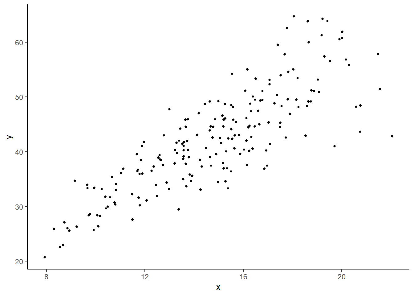
OLS estimation of this regression gives the following output.
ols <- lm(y~x, data=df_het)
sum_ols <- summary(ols)
coef(sum_ols)
cat("R-squared: ",sum_ols$r.squared,"\n")
Estimate Std. Error t value Pr(>|t|)
(Intercept) 6.285792 1.7817576 3.52786 5.207066e-04
x 2.430744 0.1177712 20.63955 3.034896e-51
R-squared: 0.6826877 Because there is obvious heteroskedasticity in this example, we should not trust the standard errors, t-statistics and p-values presented above. If we wish to stick with OLS, then we have to calculate the heteroskedasticity-robust standard errors (which we have not yet discussed how to do, except in the simple linear regression without intercept). For the time being, we will use the function vcovHC() from the sandwich package to obtain heteroskedasticity-robust standard errors (explanations in a later chapter!). The heteroskedasticity-robust standard errors are the square root of the diagonal elements of the matrix rbst_V in the example below.
rbst_V <- vcovHC(ols, type="HC0")
rbst_se <- sqrt(diag(rbst_V))
rbst_output <- coef(sum_ols)
colnames(rbst_output) <- c("Estimate", "rbst-se", "rbst-t", "p-val")
rbst_output[,'rbst-se'] <- rbst_se
rbst_output[,'rbst-t'] <- rbst_output[,'Estimate']/rbst_se
rbst_output[,'p-val'] <- 2*(1-pt(abs(rbst_output[,'rbst-t']),sum_ols$df[2]))
round(rbst_output,6)
Estimate rbst-se rbst-t p-val
(Intercept) 6.285792 1.863926 3.372339 0.000896
x 2.430744 0.136242 17.841435 0.000000Now we assume that \(\mathrm{var}[\hat{\epsilon}_i] = \sigma^2X_i^2\) and run WLS. The appropriate transformed regression is as given in Eq. 7.11.
df_het$ystar  <- df_het$y/df_het$x     # Transformed y
df_het$x0star <- 1/df_het$x            # Transformed intercept term
wls1 <- lm(ystar~x0star, data=df_het)
sum_wls1 <- summary(wls1)
coef(sum_wls1)                              # Print Coefficients
cat("R-squared: ",sum_wls1$r.squared,"\n")  # Print R-squared of Transformed Eq
Estimate Std. Error t value Pr(>|t|)
(Intercept) 2.53166 0.1023702 24.730430 1.839271e-62
x0star 4.82571 1.4065451 3.430896 7.321779e-04
R-squared: 0.05611379 Our estimated equation is \[\begin{alignat*}{4} \hat{Y} & = & 4.8257\,\, & + & 2.5317\,\, & X \,, & \quad N= 200\\ & & (1.4065)& & (0.1024) & & & \end{alignat*}\] The standard errors are lower than in the OLS regression, which is not unexpected. The R-squared in the output above refers to the fit of the transformed equation which is not very useful. We calculate the R-squared for the un-transformed regression below
ehat <- df_het$y - coef(wls1)[2] - coef(wls1)[1]*df_het$x
ssr <- sum(ehat^2)
sst <- sum((df_het$y - mean(df_het$y))^2)
R2 <- 1 - ssr/sst
cat("R-squared: ", R2,"\n")
R-squared: 0.6814966 The R-squared from the WLS regression is lower than in the OLS regression, as expected, but only slightly so. Finally, we plot the residuals from the transformed regression against \(x\). There does not appear to be any correlation between the variance of the residuals of the weighted regression and \(x\), which suggests that our assumption regarding the form of heteroskedasticity in \(\epsilon_i\) is reasonable.
plot(df_het$x, residuals(wls1))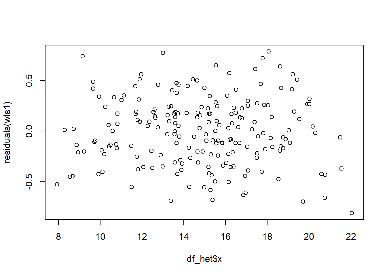
We can also use the function lm() to carry out weighted least squares. Note that the option weights refer to weights on the squared residuals, as in the \(\omega_{i}\) in Eq. 7.9.
df_het$wt <- 1/df_het$x^2
wls2 <- lm(y~x,data=df_het, weights=wt)
sum_wls2 <- summary(wls2)
coef(sum_wls2)
cat("R-squared: ", sum_wls2$r.squared,"\n")
Estimate Std. Error t value Pr(>|t|)
(Intercept) 4.82571 1.4065451 3.430896 7.321779e-04
x 2.53166 0.1023702 24.730430 1.839271e-62
R-squared: 0.755433 Notice that the R-squared provided when using lm() for WLS is different from what we previously obtained. The R-squared provided here is a “weighted R-squared”, obtained in the following way: let \(\overline{Y}_{wls}\) be the WLS estimator (with the same weights as previously) of \(\beta_0\) from the regression \(Y_i = \beta_0 + \epsilon_i\). In other words, \(\overline{Y}_{wls}\) is the weighted mean of \(\{Y_i\}_{i=1}^N\). Then \[
\text{weighted-}R^2
=
\frac{\sum_{i=1}^N w_i(\hat{Y}_{i}^{wls} - \overline{Y}_{wls})^2}
{\sum_{i=1}^N w_i(Y_{i}^{wls} - \overline{Y}_{wls})^2}\;.
\] In other words, it is the weighted ESS divided by the weighted TSS, centered on the weighted mean of \(\{Y_i\}_{i=1}^N\). We replicate the lm() weighted R-squared below:
wls0 <- lm(y~1, data=df_het, weights=wt)  # Regression on intercept only
sstw <- sum(df_het$wt * (df_het$y - coef(wls0))^2)
ssew <- sum(df_het$wt*(wls2$fitted.values - coef(wls0))^2)
WeightedR2 <- ssew/sstw
WeightedR2
[1] 0.755433The problem of specifying a form of the heteroskedasticity becomes more challenging in the multivariate regression case. Suppose \[ Y_i = \beta_0 + \beta_1 X_{1,i} + \dots + \beta_{K-1,i}X_{K-1,i} + \epsilon_i \] such that \[ \mathrm{E}[\epsilon_i^2 | \mathrm{x}_1, \dots, \mathrm{x}_{K-1}] = \sigma_i^2 = \sigma^2 \eta_i(\mathrm{x}_1, \dots, \mathrm{x}_{K-1}) \] for all \(i=1,2,...,N\). Any heteroskedasticity is likely to depend on more than one regressor, to different degrees, so there will be parameters to estimate. E.g., we might have something like \[ \eta_i = \exp(\alpha_1 X_{1,i} + \dots + \alpha_{K-1} X_{K-1,i}) \] (the exponentiation is to ensure the variance is positive). Then to implement weighted least squares, we first have to estimate the parameters in the variance equation. One way to do this is to first estimate the main equation using OLS, and obtain the OLS residuals. Then regress the log of the squared residuals on a constant and the regressors to estimate \(\sigma^2\) and the \(\alpha\) parameters, and then finally compute the “fitted variances” \(\widehat{\sigma_i^2}\) and weight the squared residuals by \(1/\widehat{\sigma_i^2}\).
7.3 Testing for Heteroskedasticity
It may be of interest to test whether heteroskedasticity is an issue in the first place. The following are some possible tests. All involve first estimating the main regression by OLS and obtaining the OLS residuals \(\hat{\epsilon}_i\).
Run the regression \[ \hat{\epsilon}_i^2 = \alpha_0 + \alpha_1X_{1,i} + \dots \alpha_{K-1}X_{K-1,i}+u_i \] and test \(H_{0}: \alpha_1 = \dots = \alpha_{K-1}=0\) using an F-test.
An alternative is to use an “LM” test after running the regression above: under the null hypothesis, we have \[ NR_{\epsilon}^2 \; \overset{a}{\sim} \; \chi_{(K)}^2. \]
To allow for possible non-linear forms we can include powers of regressors and interaction terms between them in the variance regression: \[ \begin{aligned} \hat{\epsilon}_i^2 = \alpha_0 &+ \alpha_1X_{1,i} + \dots + \alpha_{K-1}X_{K-1,i} \\ &+ \delta_1X_{1,i}^2 + \dots + \delta_{K-1}X_{K-1,i}^2 \\ &+ \gamma_{12} X_{1,i}X_{2,i} + \dots + u_i \end{aligned} \] then testing if all of the coefficients (not including the intercept) are zero. Obviously you lose degrees of freedom quickly as the number of regressors grow.
One way around this problem is to run the regression \[ \hat{\epsilon}_i^2 = \alpha_0 + \alpha_1\hat{Y}_{i,ols} + \alpha_{2}\hat{Y}_{i,ols}^2 + u_i \] where \(\hat{Y}_{i,ols}\) refers to the OLS fitted values from the main equation. The hypothesis that there is no heteroskedasticity is \(H_0: \alpha_1 = \alpha_2 = 0\) using an F-tests or an LM test.
The first two is often referred to as Breusch-Pagan tests for heteroskedasticity. The last is referred to as the White test for heteroskedasticity.
Example 7.4 We apply the Breusch-Pagan test for heteroskedasticity to the regression \[ ln(earnings_i) = \beta_0 + \beta_1 wexp_i + \beta_2 tenure_i + \epsilon_i. \]
df_earn <- read_excel("data\\earnings.xlsx")        #--Read Data
mdl <- lm(log(earnings)~wexp+tenure, data=df_earn)  #--Main Equation
cat("Main Regression\n")                            #--Main Regr Output Title
round(summary(mdl)$coefficients,4)                  #--Main Regr Output
Main Regression
Estimate Std. Error t value Pr(>|t|)
(Intercept) 2.4734 0.0980 25.2385 0.0000
wexp 0.0127 0.0060 2.1294 0.0337
tenure 0.0147 0.0041 3.5596 0.0004df_earn$ehat <- residuals(mdl) #--Get OLS Residuals
heteq <- lm((ehat^2)~wexp+tenure, data=df_earn) #--BP-Test Regression
cat("Heteroskedasticity Test Regression\n") #--Test Regr Output Title
round(summary(heteq)$coefficients,4) #--Test Regr OutputHeteroskedasticity Test Regression
Estimate Std. Error t value Pr(>|t|)
(Intercept) 0.5596 0.0927 6.0375 0.0000
wexp -0.0121 0.0057 -2.1471 0.0322
tenure -0.0035 0.0039 -0.8877 0.3751## BP, F-version
f_het <- summary(heteq)$fstatistic #--Retrieve F-Stat (stat, df1, df2)
cat("BP-F Stat: ", f_het[1], " p-val: ", 1-pf(f_het[1], f_het[2], f_het[3]), "\n") BP-F Stat: 3.855297 p-val: 0.02175567 ## BP, LM-version
lm_het <- nobs(heteq)*summary(heteq)$r.squared # Calc. LM Stat.
lm_pval <- 1 - pchisq(lm_het, 2) # 2 restrictions
cat("BP-LM Stat: ", lm_het, " p-val: ", lm_pval, "\n", sep="")BP-LM Stat: 7.643914 p-val: 0.02188493There is some evidence of heteroskedasticity, and the individual t-tests suggest that the noise variance decreases with work experience.
7.4 Some Additional Regression Tests
We mention a few other tests associated with regressions.
7.4.1 RESET test for functional form misspecification
Given a regression specification \[ Y_i = \beta_{0} + \beta_{1} X_{1,i} + \dots + \beta_{K-1} X_{K-1,i} + \epsilon_i\,, \] the Regression Equation Specification Error Test (or “RESET Test”) checks if adding powers (\(X_{1,i}^2\), \(X_{2,i}^2\),…) and interaction terms (\(X_{1,i}X_{2,i}\), \(X_{1,i}X_{3,i}\), etc.) of the regressors can significantly improve the fit. It is interpreted as a test of adequacy of the functional form specification of the original regression, and not as saying anything about the whether or not certain variables should or should not be included. Similar to the White test for heteroskedasticity, the RESET test does this by adding the squares, cubes, and possibly higher powers of the OLS fitted values \(\hat{Y}_{i,ols}\) into the regression specification and tests if these additions have significant explanatory power, i.e., the test equation is \[ Y_i = \beta_{0} + \beta_{1} X_{1,i} + \dots + \beta_{K-1} X_{K-1,i} + \alpha_2\hat{Y}_{i,ols}^2 + \dots + \alpha_p\hat{Y}_{i,ols}^p + \epsilon_i\,, \tag{7.12}\] and the hypothesis of adequacy of the functional form specification is \[ H_0: \alpha_2 = \dots = \alpha_p = 0. \] The test equation cannot include \(\hat{Y}_{i,ols}\) (see exercises), and often only the second or second and third powers are included. An F-test (or t-test, if only the second power is included) can be used to test the hypothesis. We illustrate the RESET test in the next example.
Example 7.5 We apply the RESET test to the regression \[
\ln(earnings_i) = \beta_0 + \beta_1 wexp_i + \beta_2 tenure_i + \epsilon_i.
\] using data in earnings.xlsx.
df_earn <- read_excel("data\\earnings.xlsx")
mdl_base <- lm(log(earnings)~wexp+tenure, data=df_earn)
df_earn$yhat <- fitted(mdl_base)
mdl_test <- lm(log(earnings)~wexp+tenure+I(yhat^2), data=df_earn)
cat("Base Regression:\n")
round(summary(mdl_base)$coefficients, 4)
cat("\nTest Regression:\n")
round(summary(mdl_test)$coefficients, 4)
Base Regression:
Estimate Std. Error t value Pr(>|t|)
(Intercept) 2.4734 0.0980 25.2385 0.0000
wexp 0.0127 0.0060 2.1294 0.0337
tenure 0.0147 0.0041 3.5596 0.0004
Test Regression:
Estimate Std. Error t value Pr(>|t|)
(Intercept) 23.4033 8.3837 2.7915 0.0054
wexp 0.2544 0.0970 2.6233 0.0090
tenure 0.3069 0.1171 2.6206 0.0090
I(yhat^2) -3.4656 1.3881 -2.4967 0.0128The hypothesis of adequacy of the functional form in the base regression is rejected.
7.4.2 Testing Nonnested Alternatives
Regression specifications such as \[ \begin{aligned} &\text{[A]} \quad Y_i = \beta_0 + \beta_1X_{1,i} + \beta_2 X_{2,i} + \epsilon_i \\ \text{and} \quad &\text{[B]} \quad Y_i = \beta_0 + \beta_1\ln X_{1,i} + \beta_2 \ln X_{2,i} + \epsilon_i \end{aligned} \] are “non-nested alternatives”, i.e., one is not a special case of the other. One way of testing which specification fits better is to construct a “super-model” that includes both [A] and [B] as restricted cases, i.e., \[ \text{[A]} \quad Y_i = \beta_0 + \beta_1X_{1,i} + \beta_2 X_{2,i} + \beta_3 \ln X_{1,i} + \beta_4 \ln X_{2_i} + \epsilon_i \] and to test for coefficient significance. This approach is often plagued by multicollinearity problems. An alternative is to fit both models separately, collect their fitted values, and include each fitted value series as a regressor in the other specification, i.e., regress \[ \begin{aligned} &\text{[A']} \quad Y_i = \beta_0 + \beta_1X_{1,i} + \beta_2 X_{2,i} + \delta_1 \hat{Y}_i^B + \epsilon_i \\ \text{and} \quad &\text{[B']} \quad Y_i = \beta_0 + \beta_1\ln X_{1,i} + \beta_2 \ln X_{2,i} + \delta_2 \hat{Y}_i^A + \epsilon_i \end{aligned} \] and test (separately) if the coefficients on the fitted values are statistically significant. The idea is to see if each specification has anything to add to the other. If \(\delta_1=0\) is rejected and \(\delta_2=0\) is not, then this suggests that [B] is a better specification (the result does not suggest [B] is the best specification, just better than [A].) Likewise, [A] is preferred to [B] if \(\delta_2=0\) is rejected and \(\delta_1=0\) is not. It may be that both are rejected, which suggests that neither specification is adequate. If neither are rejected, then it appears that there is little in the data to distinguish between the two specifications. Note that the dependent variable in both alternatives must be the same.
We compare the specifications \[ \begin{aligned} &\text{[A]} \quad \ln(earnings_i) = \beta_0 + \beta_1 wexp_i + \beta_2 tenure_i + \epsilon_i \\ \text{and} \quad &\text{[B]} \quad \ln(earnings_i) = \beta_0 + \beta_1 \ln(wexp_i) + \beta_2 \ln(tenure_i) + \epsilon_i\,. \end{aligned} \]
mdlA <- lm(log(earnings)~wexp+tenure, data=df_earn)
mdlB <- lm(log(earnings)~log(wexp)+log(tenure), data=df_earn)
df_earn$yhatA <- fitted(mdlA)
df_earn$yhatB <- fitted(mdlB)
cat("Model A plus yhatB:\n")
mdlAplusB <- lm(log(earnings)~wexp+tenure+yhatB, data=df_earn)
round(summary(mdlAplusB)$coefficients,4)
cat("\nModel B plus yhatA:\n")
mdlBplusA <- lm(log(earnings)~log(wexp)+log(tenure)+yhatA, data=df_earn)
round(summary(mdlBplusA)$coefficients,4)
Model A plus yhatB:
Estimate Std. Error t value Pr(>|t|)
(Intercept) -0.1193 0.8700 -0.1371 0.8910
wexp -0.0030 0.0079 -0.3747 0.7080
tenure 0.0000 0.0064 -0.0024 0.9981
yhatB 1.0607 0.3537 2.9990 0.0028
Model B plus yhatA:
Estimate Std. Error t value Pr(>|t|)
(Intercept) 2.3694 0.9658 2.4534 0.0145
log(wexp) 0.1671 0.0962 1.7375 0.0829
log(tenure) 0.0925 0.0326 2.8386 0.0047
yhatA -0.0606 0.4121 -0.1471 0.8831It appears that the specification [B] is preferred over specification [A].
7.4.3 Testing for Normality of Noise Terms
The finite sample justification for the t- and F-tests depend on the normality of the noise terms. One way to test this is to use the fact that if a random variable has the normal distribution, then its skewness coefficient is zero (because it is symmetric), and its kurtosis coefficient is three: if \(X \sim \text{Normal}(\mu, \sigma^2)\), then \[ \begin{gathered} S = \mathrm{E}[(X-\mu)^3]/\sigma^3 = 0 \\ Kur = \mathrm{E}[(X-\mu)^4]/\sigma^4 = 3\,. \end{gathered} \] The kurtosis coefficient, being the expectation of a fourth moment, emphasizes larger deviations from mean over small deviations from mean (deviations from mean less than one become very small when raised to the fourth power). A kurtosis coefficient greater than 3 suggests higher probability of large deviations from mean, relative to a comparable normally distributed random variable. The skewness and kurtosis coefficients can be estimated using \[ \begin{aligned} \widehat{S} &= \frac{\frac{1}{N}\sum_{i=1}^N(X_i-\overline{X})^3} {\left[\frac{1}{N}\sum_{i=1}^N(X_i-\overline{X})^2\right]^{3/2}} \\ \widehat{Kur} &= \frac{\frac{1}{N}\sum_{i=1}^N(X_i-\overline{X})^4} {\left[\frac{1}{N}\sum_{i=1}^N(X_i-\overline{X})^2\right]^{2}} \,. \end{aligned} \] The Jarque-Bera statistic applies this idea to regression residuals, using the statistic \[ JB = \frac{N-K}{6}\left(\hat{S}^2 + \frac{1}{4}(\widehat{Kur} - 3)^2\right) \] which is approximately \(\chi_{(2)}^2\) in large samples under the null. Some implementations ignore the degree-of-freedom correction and use \(N\) in the numerator instead of \(N-K\).
We test for normality of the residuals in the regression \[ \ln(earnings) = \beta_0 + \beta_1 \ln(wexp_i) + \beta_2 \ln(tenure_i) + \epsilon_i \]
Skew <- function(x){
  # Returns Skewness Coefficient
  return(mean((x-mean(x))^3)/(mean((x-mean(x))^2)^(3/2)))
}
Kurt <- function(x){
  # Returns Kurtosis Coefficient
  return(mean((x-mean(x))^4)/(mean((x-mean(x))^2)^2))
}
JB <- function(mdl){
  # requires lm object, returns JB Stat, p-val, Skewness and Kurtosis Coef.
  N <- nobs(mdl)
  K <- summary(mdl)$df[1]
  ehat <- residuals(mdl)
  JBSkew <- Skew(ehat)
  JBKurt <- Kurt(ehat)
  JBstat <- ((N-K)/6*(JBSkew^2 + (1/4)*(JBKurt-3)^2))
  JBpval <- 1-pchisq(JBstat,2)
  return(list("JBstat"=JBstat,
              "JBpval"=JBpval,
              "Skewness"=JBSkew,
              "Kurtosis"=JBKurt))
}
df_earn <- read_excel("data\\earnings.xlsx")
mdl <- lm(log(earnings)~log(wexp)+log(tenure), data=df_earn)
JBtest <- JB(mdl)
fmt <- function(x){format(round(x,4),nsmall=4)}
cat("JB:", fmt(JBtest$JBstat),
    "  p-val:", fmt(JBtest$JBpval),
    "  Skewness:", fmt(JBtest$Skewness),
    "  Kurtosis:", fmt(JBtest$Kurtosis),"\n")
JB: 40.8122 p-val: 0.0000 Skewness: 0.4470 Kurtosis: 4.0123 The null of normality is rejected. There appears to be a slight skewness to the right, and ‘excess kurtosis’ (kurtosis in excess of 3). A histogram of the OLS residuals is shown below.
hist(residuals(mdl), 20)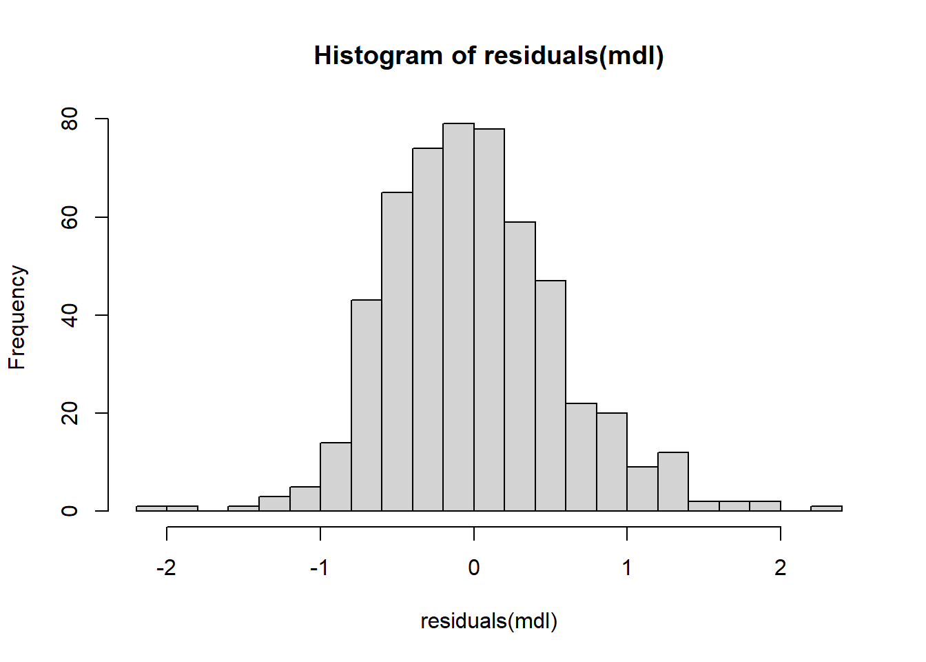
7.5 Exercises
Exercise 7.1 Show in Example 7.1 that the modified noise terms are uncorrelated, i.e., \[ \mathrm{E}[\epsilon_i^*\epsilon_j^* | \mathrm{x}] = 0 \] for all \(i \neq j\); \(i,j=1,2,...,N\).
Exercise 7.2 In the notes we claimed that \[ \frac{\sum_{i=1}^N X_i^4}{\left(\sum_{i=1}^N X_i^2\right)^2} \geq \frac{1}{N}. \] Prove this by showing that for any set of values \(\{z_i\}_{i=1}^N\), we have \[ N\sum_{i=1}^N z_i^2 - \left( \sum_{i=1}^N z_i\right)^2 \geq 0. \] (Hint: start with the fact that \(\sum_{i=1}^N(z_i - \bar{z})^2 \geq 0\).) Then substitute \(X_i^2\) for \(z_i\). When will equality hold?
Exercise 7.3
Calculate the heteroskedasticity-robust standard errors for the regression in Example 7.4. Compare the robust standard errors with the OLS standard errors.
Estimate (using
lm()) the main equation in Example 7.4 using WLS, assuming \[ \mathrm{var}[\epsilon_i|\mathrm{wexp}, \mathrm{tenure}] = \sigma^2 wexp_i\,. \] Compare the WLS estimation results with the OLS estimation results (with heteroskedasticity robust standard errors).
Exercise 7.4
Why is it that we cannot include \(\hat{Y}_{i,ols}\) in the RESET test equation?
Add the third power of the OLS fitted value in the RESET test equation in Example 7.5. What happens to the statistical significance of the original regressors? Can you explain the likely cause? Hint: what is the correlation between
yhat^2andyhat^3?