library(tidyverse)
library(patchwork)
library(latex2exp)3 Probability and Expectations Review
We describe the outcomes of “experiments” as random variables. By “experiment”, we mean any sort of activity (human or otherwise) that can result in a range of outcomes, and such that which outcomes occur can be thought of (at some level) as random. This chapter contains a few examples to review the idea of random variables and related concepts. The R code in this chapter uses the tidyverse and patchwork packages.
3.1 Random Variables, Mean and Variance
For our first example, suppose there are two urns A and B each containing 100 balls numbered 1 to 10. We will call a ball that is numbered \(i\) an “\(i\)-ball” (so we have 1-balls, 2-balls, 3-balls, and so on). The number of \(i\)-balls in each urn is shown below.
UrnA <- c(3, 4, 8, 15, 20, 20, 15, 8, 4, 3);
UrnB <- c(16, 50, 16, 8, 4, 2, 1, 1, 1, 1);
ballnum = 1:10
ballnames <- paste0(ballnum,"-Ball")
names(UrnA) <- ballnames
names(UrnB) <- ballnames
cat("Urn A:\n"); UrnA
cat("Urn B:\n"); UrnB
Urn A:
1-Ball 2-Ball 3-Ball 4-Ball 5-Ball 6-Ball 7-Ball 8-Ball 9-Ball 10-Ball
3 4 8 15 20 20 15 8 4 3
Urn B:
1-Ball 2-Ball 3-Ball 4-Ball 5-Ball 6-Ball 7-Ball 8-Ball 9-Ball 10-Ball
16 50 16 8 4 2 1 1 1 1 Suppose you pick one ball at random from Urn A (suppose the balls are well mixed, you don’t look, etc.). It seems reasonable to think that the chance, or probability, of drawing a 1-ball, 2-ball, 3-ball, etc. is 0.03, 0.04, 0.08, and so on. If \(X\) be the number on the ball that is drawn, then \(X\) is a random variable, with probability distribution function (pdf) \(p(x) = Pr[X=x]\) as shown in Fig. 3.1(a) below. Likewise, if \(Y\) is the number on a ball drawn from Urn B, then it too is a random variable, with pdf as shown in Fig. 3.1(b).
pdfX = data.frame(x=ballnum, probx=UrnA/100)
pdfY = data.frame(y=ballnum, proby=UrnB/100)
my_theme <- theme_bw() + theme(axis.title=element_text(size=10), aspect.ratio = 0.8)
p1 <- pdfX %>% mutate(x=as.factor(x)) %>% ggplot(aes(x=x, y=probx)) + ggtitle("Urn A") +
  geom_bar(stat="identity", width=0.2) + ylim(0,0.52) + ylab("P(X=x)") + my_theme
p2 <- pdfY %>% mutate(y=as.factor(y)) %>% ggplot(aes(x=y, y=proby)) + ggtitle("Urn B") +
  geom_bar(stat="identity", width=0.2) + ylim(0,0.52) + ylab("P(Y=y)") + my_theme
(p1|p2)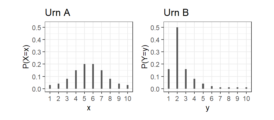
It seems the “central location” as well as the “spread” of the two probability distributions are quite different. Can we come up with What indicators can we use to describe these features?
Suppose a random variable \(X\) takes possible values \(x_{i}\) with probabilities \(p(x_{i})=\Pr[X=x_{i}]\), \(i=1,2,...,N\). For central location the following indicators are popular: \[ \begin{aligned} \text{mean:} \quad E[X] &= \sum_{i=1}^{N} x_{i}\Pr[X=x_{i}]\;, \\ \text{median:} \quad \text{mdn}[X] &= m \;\; \text{such that}\;\; \Pr[X\leq m] = 0.5 \;\text{ and }\; \Pr[X\geq m] = 0.5\;, \\[10pt] \text{mode:} \quad \text{mo}[X] &= x_{j} \;\;\text{such that}\;\; \Pr[X=x_{j}] \geq \Pr[X=x_{i}] \;\; \text{for all}\;\; i=1,2,...,N\;. \end{aligned} \tag{3.1}\] The definitions are for a random variable taking \(n\) possible values. Later we extend the definition to other kinds of random variables.
The mean, also called the expected value, is a weighted average. Imagine that the probabilities are weights resting on a plank under which you place a pivot. The mean is the location of the pivot such that the probabilities on either side balances and the plank rests horizontally on the pivot. For this reason, the mean is called a moment. For out random variables:
mu_X <- sum(pdfX$x*pdfX$probx)
mu_Y <- sum(pdfY$y*pdfY$proby)
cat("E[X] =", round(mu_X,3), "and E[Y] =", round(mu_Y,3), ".")
E[X] = 5.5 and E[Y] = 2.62 .The definition of the mean is easy to extend to functions of \(X\), e.g., the mean of \(g(X)\) is just \[ E[g(X)] = \sum_{i=1}^{N} g(x_{i})\Pr[X=x_{i}]\;. \tag{3.2}\]
The median is a value such that the probabilities on either side of it add to 0.5. One problem with this measure is that there may be many values or none (for \(X\), all values from 5 to 6 inclusive are medians, and we cannot calculate the median of \(Y\)). The mode is a value that has the highest probability. Again, the mode may not be unique. The mode of \(Y\) is 2, but the modes of \(X\) are 5 and 6.
For spread, a popular indicator is the variance: \[ \begin{aligned} \text{variance:} \quad var[X] &= \sum_{i=1}^{n} (x_{i}-E[X])^{2}\Pr[X=x_i] \\ &= E[(X-E[X])^{2}]\,. \end{aligned} \tag{3.3}\] The second line in Eq. 3.3 is just a restatement of the first, using the definition of an expectation.
The variance is the probability-weighted average of the squared deviations of the possible values from the mean. If the bulk of the probabilities are on values near the mean, then small \((x_{i}-E[X])^{2}\) will be given more weight and the variance will be smaller. For our random variables:
var_X <- sum((pdfX$x-mu_X)^2*pdfX$probx)
var_Y <- sum((pdfY$y-mu_Y)^2*pdfY$proby)
cat("var[X] =", round(var_X,3), "and var[Y] =", round(var_Y,3), ".")
var[X] = 3.97 and var[Y] = 2.676 .Expanding the square in Eq. 3.3, we get an alternative way of computing the variance: \[ \begin{aligned} \sum_{i=1}^{n} (x_{i}-E[X])^{2}&\Pr[X=x_i] = \sum_{i=1}^{n} (x_{i}^{2}-2E[X]x_{i} + E[X]^2)\Pr[X=x_i] \\ &= \sum_{i=1}^{n} x_{i}^{2}\Pr[X=x_i] - 2E[X]\sum_{i=1}^{n}x_{i}\Pr[X=x_i] + E[X]^2\sum_{i=1}^{n}Pr[X=x_i] \\ &= \sum_{i=1}^{n} x_{i}^{2}\Pr[X=x_i] - 2E[X]^{2} + E[X]^2 \\[8pt] &= E[X^{2}] - E[X]^{2} \end{aligned} \tag{3.4}\] This version is often easier to use. The variance is also known as the “second central moment”. The square root of the variance is the standard deviation. There are other measures such as the “inter-quartile range” but we won’t be using these.
The mean and variance are popular measures because they are easy to work with and manipulate. For instance, it is easy to show from the definitions of the mean and variance in Eq. 3.1 and Eq. 3.3 that for any random variable \(X\), we have
- \(E[aX+b] = a E[X] + b\)
- \(var[aX+b] = a^{2} var[X]\)
These are left as an exercise.
Suppose the game is: you get to pick one ball from one urn, and you win in dollars 100 times the number on the ball. To pick from Urn A, you first have to pay $500. To pick from Urn B, you only pay $250. Which urn would you choose to play, or would you not play? (Just asking.)
3.2 Joint and Conditional Distributions
Suppose you live in a place with no seasons, and seemingly random variations in temperature and precipitation from day to day, with the following probabilities.
Weather = matrix(c(0.05, 0.15, 0.35, 0.10, 0.15, 0.20), nrow=2, byrow=T)
colnames(Weather) <- c("Cool", "Warm", "Hot")
rownames(Weather) <- c("Dry", "Rainy")
cat("Joint Probability Distribution of Temperature and Precipitation:\n")
Weather
SumWeather <- sum(Weather)
cat("Total Probabilities = ", SumWeather)
Joint Probability Distribution of Temperature and Precipitation:
Cool Warm Hot
Dry 0.05 0.15 0.35
Rainy 0.10 0.15 0.20
Total Probabilities = 1This is an example of a joint probability distribution1 for two variables: Temperature (Temp) taking values ‘Cool’, ‘Warm’ and ‘Hot’, and Precipitation (Prcp) taking values ‘Dry’ and ‘Rainy’. It gives the probabilities of joint Temperature-Precipitation events like ‘Cool and Rainy’, ‘Hot and Dry’, and so on. In notation \[ \Pr[\text{Temp}=\text{Cool}, \text{Prcp}=\text{Dry}] = 0.05\,,\,\,\Pr[\text{Temp}=\text{Warm}, \text{Prcp}=\text{Rainy}] = 0.15, \text{ etc.} \] with probabilities adding to one. So, out of every hundred days, we should see about 20 Hot and Rainy days, 5 Cool and Dry days, etc. In what follows, I will just write \(\Pr[\text{Cool}, \text{Dry}]\) for \(\Pr[\text{Temp}=\text{Cool}, \text{Prcp}=\text{Dry}]\).
What is the probability of Dry days (regardless of temperature)? “Dry regardless of temperature” means Dry & Cool, Dry & Warm, and Dry & Hot all count, so we add up the probabilities in the first row to get \(\Pr[\text{Dry}]=0.55\). Likewise, \(\Pr[\text{Rainy}]=0.45\). These two probabilities make up the marginal, or unconditional, probability distribution for Precipitation. To get the marginal or unconditional probability distribution for Temperature, we add up the columns. We get: \(\Pr[\text{Cool}]=0.15\), \(\Pr[\text{Warm}]=0.3\), \(\Pr[\text{Hot}]=0.55\). We show these two marginal distributions in the last column and row of the table below:
cat("Joint and Marginal Probability Distribution of Prec and Temp:\n")
MargPrcp <- rowSums(Weather)
MargTemp <- colSums(Weather)
WeatherWithMarg <- cbind(Weather, MargPrcp)
WeatherWithMarg <- rbind(WeatherWithMarg, MargTemp=c(MargTemp, SumWeather) )
WeatherWithMarg
Joint and Marginal Probability Distribution of Prec and Temp:
Cool Warm Hot MargPrcp
Dry 0.05 0.15 0.35 0.55
Rainy 0.10 0.15 0.20 0.45
MargTemp 0.15 0.30 0.55 1.00We can ask a different sort of question about the weather in this place. E.g., what is the precipitation like on Cool days? From the “Cool” column in the joint distribution, we see that on Cool days it is twice as likely to be Rainy than Dry. We want to describe precipitation on Cool days as a probability distribution, and total probabilities must add to one, so we divide the “Cool” column of the joint distribution by \(\Pr[\text{Cool}]\). This gives the Conditional Probability Distribution of Precipitation given Temperature = Cool. In notation: \[ \begin{aligned} \Pr[\,\text{Dry}\,| \,\text{Cool}\,] &= \frac{\Pr[\,\text{Dry},\,\text{Cool}\,]}{\Pr[\,\text{Cool}\,]} = \frac{0.05}{0.15} = 1/3 \\[8pt] \Pr[\,\text{Rainy}\,|\,\text{Cool}\,] &= \frac{\Pr[\,\text{Rainy},\,\text{Cool}\,]}{\Pr[\,\text{Cool}\,]} = \frac{0.1}{0.15} = 2/3 \end{aligned} \tag{3.5}\] We can make similar calculations for Warm and Hot days to get the conditional distributions for Precipitation given Temperature = Warm, and given Temperature = Hot. All three conditional distributions are shown in the columns of the output below:
PrcpGivenTemp = Weather
PrcpGivenTemp[, 'Cool'] <- Weather[, 'Cool'] / MargTemp['Cool']
PrcpGivenTemp[, 'Warm'] <- Weather[, 'Warm'] / MargTemp['Warm']
PrcpGivenTemp[, 'Hot'] <- Weather[, 'Hot'] / MargTemp['Hot']
rownames(PrcpGivenTemp) <- c("Pr[Dry|Temp]", "Pr[Rainy|Temp]")
cat("Conditional Distribution of Precipitation Given Temperature (columns):\n")
round(PrcpGivenTemp,3)
Conditional Distribution of Precipitation Given Temperature (columns):
Cool Warm Hot
Pr[Dry|Temp] 0.333 0.5 0.636
Pr[Rainy|Temp] 0.667 0.5 0.364On warm days, it is fifty-fifty whether it is Dry or Rainy. On Hot days, it is more likely to be Dry than Rainy. We emphasize that each column is a distribution, so the conditional distribution of Precipitation given Temperature is really a collection of three distribution different distributions.
Similar calculations gives the conditional distribution of Temperature given Precipitation, e.g., what are the probabilities each of Cool, Warm, and Hot days given it is Dry? By the same reasoning as before, \[ \begin{gathered} \Pr[\,\text{Cool}\,|\,\text{Dry}\,] = \frac{\Pr[\,\text{Dry},\,\text{Cool}\,]}{\Pr[\,\text{Dry}\,]} = \frac{0.05}{0.55} = 1/11 \\[8pt] \Pr[\,\text{Warm}\,|\,\text{Dry}\,] = \frac{\Pr[\,\text{Dry},\,\text{Warm}\,]}{\Pr[\,\text{Dry}\,]} = \frac{0.15}{0.55} = 3/11 \\[8pt] \Pr[\,\text{Hot}\,|\,\text{Dry}\,] = \frac{\Pr[\,\text{Dry},\,\text{Hot}\,]}{\Pr[\,\text{Dry}\,]} = \frac{0.35}{0.55} = 7/11 \\ \end{gathered} \tag{3.6}\] Likewise for Rainy days. The two conditional distributions of temperature given precipitation are shown in the rows of the output below, with probabilities rounded to 3 decimal places.
TempGivenPrcp = Weather
TempGivenPrcp['Dry',] <- Weather['Dry',] / MargPrcp['Dry']
TempGivenPrcp['Rainy',] <- Weather['Rainy',] / MargPrcp['Rainy']
colnames(TempGivenPrcp) <- c("Pr[Cool|Prcp]","Pr[Warm|Prcp]","Pr[Hot|Prcp]")
cat("Conditional Distribution of Temperature Given Precipitation (rows):\n")
round(TempGivenPrcp,3)
Conditional Distribution of Temperature Given Precipitation (rows):
Pr[Cool|Prcp] Pr[Warm|Prcp] Pr[Hot|Prcp]
Dry 0.091 0.273 0.636
Rainy 0.222 0.333 0.4443.2.1 Bayes’ Theorm
There is a tidy relationship between the conditional distributions. From the first equations of Eq. 3.5 and Eq. 3.6, we can deduce that \[ \Pr[\,\text{Dry}\,|\,\text{Cool}\,]\,\Pr[\,\text{Cool}\,] = \Pr[\,\text{Cool}\,|\,\text{Dry}\,]\,\Pr[\,\text{Dry}\,]\;, \] since both are equal to \(\Pr[\,\text{Cool},\,\text{Dry}\,]\). It follows that \[ \Pr[\,\text{Dry}\,|\,\text{Cool}\,] = \frac{\Pr[\,\text{Cool}\,|\,\text{Dry}\,]\Pr[\,\text{Dry}\,]}{\Pr[\,\text{Cool}\,]} \,. \tag{3.7}\] In our example, we found that \(\Pr[\,\text{Dry}\, | \,\text{Cool}\,] = 1/3\) whereas \(\Pr[\,\text{Cool}\, | \,\text{Dry}\,] = 1/11\) which goes to show that the two can be very different. Furthermore we can verify that \(1/3 = ((1/11) \times 0.55)/0.15\), where \(\Pr[\,\text{Dry}\,] = 0.55\) and \(\Pr[\,\text{Cool}\,] = 0.15\).
Since \[ \begin{aligned} \Pr[\,\text{Cool}\,] &= \Pr[\,\text{Cool},\,\text{Dry}\,] + \Pr[\,\text{Cool},\,\text{Rainy}\,] \\ &= \Pr[\,\text{Cool}\,|\,\text{Dry}\,] \Pr[\,\text{Dry}\,] + \Pr[\,\text{Cool}\,|\,\text{Rainy}\,]\Pr[\,\text{Rainy}\,]\,, \end{aligned} \] another version of Eq. 3.7 is \[ \Pr[\,\text{Dry}\, | \,\text{Cool}\,] = \frac{\Pr[\,\text{Cool}\, | \,\text{Dry}\,]\Pr[\,\text{Dry}\,]} {\Pr[\,\text{Cool}\, | \,\text{Dry}\,]\Pr[\,\text{Dry}\,] + \Pr[\,\text{Cool}\, | \,\text{Rainy}]\Pr[\,\text{Rainy}\,]}\,. \] You can write similar equations for the other combinations of temperature and precipitation.
Eq. 3.7 is an example of Bayes’ Theorem. If \(A\) and \(B\) are two events such that \(\Pr[A] \neq 0\) and \(\Pr[B] \neq 0\), then \[ \Pr[A|B] = \frac{\Pr[B|A] \Pr[A]}{\Pr[B]}\,. \] Likewise, we have \[ \Pr[B|A] = \frac{\Pr[A|B] \Pr[B]}{\Pr[A]}\,. \]
The following example might be a helpful illustration of the theorem.
Example 3.1 Imagine that an infectious disease enters a population of 101,000 people but that a large percentage – 100,000 out of 101,000 members of the population have vaccinated themselves against this disease. Of the 1000 not vaccinated, 50 percent (500 people) caught the disease. Only one percentage of these 100,000 vaccinated people (1000 people) eventually caught the disease, so the vaccine is effective.
Of those that caught the disease, more were vaccinated than un-vaccinated, but this is simply because a large proportion of the population received the vaccine, and 1 percent of 100,000 is more than 50 percent of 1000. The proportion of those that caught the disease being vaccinated (1000 out of 1500, or 0.67) is analogous to the probability of having been vaccinated conditional on catching the disease, \(\Pr[\,\text{vaccinated}\,|\,\text{infected}\,]\), but this proportion doesn’t say much about the effectiveness of the vaccine, if that is what we are interested in. What we want instead is the probability of being infected conditional on being vaccinated, i.e., \(\Pr[\text{infected}|\text{vaccinated}]\), which is \(1000/100,000\).
How do we get from \[ \Pr[\,\text{vaccinated}\,|\,\text{infected}\,] = \frac{1000}{1500} \quad \text{to} \quad \Pr[\,\text{infected}\,|\,\text{vaccinated}\,] = \frac{1000}{100,000} \;? \] If we multiply by the ratio of the percentage of the population that caught the disease \(\Pr[\,\text{infected}\,]\) to the percentage of those who got vaccinated \(\Pr[\,\text{vaccinated}\,]\), then \[ \begin{aligned} \Pr[\,\text{infected}\,|\,\text{vaccinated}\,] &= \frac{\Pr[\,\text{vaccinated}\,|\,\text{infected}\,] \Pr[\,\text{infected}\,]} {\Pr[\,\text{vaccinated}\,]} \\ &= \frac{\frac{1000}{1500}\frac{1500}{101,000}}{\frac{100,000}{101,000}} = \frac{1000}{100000} = 0.01\,. \end{aligned} \]
3.2.2 Mean and Variance, Covariance
At this point we cannot calculate things like means and variance for precipitation and temperature because we have only expressed the outcomes as categories, not quantities. Suppose Dry = 0mm of rain per day, and Rainy = 30mm of rain per day, and Hot=\(34\) deg C, Warm=\(28\)C and Cool=\(22\)C. Then the joint distribution is \[ p(temp, prcp) = \Pr[\,\text{Temp}=temp\,,\, \text{Prcp}=prcp\,]\;, \] where \(temp = 22, 28, 34\) and \(prcp = 0,30\), as defined in the table below:
prcp <- c(0,30); temp <- c(22, 28, 34)
rownames(Weather) <- paste0(prcp, "mm"); colnames(Weather) <- paste0(temp, "C")
cat("Joint Distribution Pr[Temp = temp, Prcp = prcp]\n")
Weather
Joint Distribution Pr[Temp = temp, Prcp = prcp]
22C 28C 34C
0mm 0.05 0.15 0.35
30mm 0.10 0.15 0.20The marginal distributions are
names(MargPrcp) <- NULL
tbl <- cbind(prcp, MargPrcp); colnames(tbl) <- c("prcp(mm)", "Pr[Prcp=prcp]"); tbl
cat("\n")
names(MargTemp) <- NULL
tbl <- cbind(temp, MargTemp); colnames(tbl) <- c("temp(C)", "Pr[Temp=temp]"); tbl
prcp(mm) Pr[Prcp=prcp]
[1,] 0 0.55
[2,] 30 0.45
temp(C) Pr[Temp=temp]
[1,] 22 0.15
[2,] 28 0.30
[3,] 34 0.55From these we can calculate the mean and variance of Prcp and Temp:
muPrcp <- sum(prcp*MargPrcp); muTemp <- sum(temp*MargTemp)
varPrcp <- sum((prcp-muPrcp)^2*MargPrcp); varTemp <- sum((temp-muTemp)^2*MargTemp)
cat("  E[Prcp] =", muPrcp, "mm"); cat("           "); cat("  E[Temp] =", muTemp, "C\n");
cat("var[Prcp] =", varPrcp, "sqr mm"); cat("     "); cat("var[Temp] =", varTemp, "sqr C\n");
cat(" sd[Prcp] =", round(sqrt(varPrcp),2), "mm"); cat("          ");
cat(" sd[Temp] =", round(sqrt(varTemp),2), "C")
E[Prcp] = 13.5 mm E[Temp] = 30.4 C
var[Prcp] = 222.75 sqr mm var[Temp] = 19.44 sqr C
sd[Prcp] = 14.92 mm sd[Temp] = 4.41 CNote the units of measurements on these moments, which are often not included when the moments are reported.
Do you notice a negative relationship between temperature and precipitation? One indicator of such an association is the covariance between two variables \(X\) and \(Y\) defined as \[ \begin{aligned} cov[X,Y] &= \sum_{i=1}^{N} \sum_{j=1}^{M} (x_{i} - E[X])(y_{j}-E[Y]) \Pr[X=x_{i}, Y=y_{j}] \\ &= E[(X-E[X])(Y-E[Y])] \\[8pt] &= E[XY] - E[X]E[Y]\, \end{aligned} \tag{3.8}\] where we assume \(X\) has \(N\) possible values and \(Y\) has \(M\) possible values. The second expression is just a restatement of the first. Notice that the “outer” expectation is with respect to the joint probabilities. To make this clear, we might write \[ cov[X,Y] = E_{X,Y}[(X-E_{X}[X])(Y-E_{Y}[Y])]\,, \] but the subscripts are usually omitted. For \(E_{X}[X]\) and \(E_{Y}[Y]\), it doesn’t matter whether you use the marginal or joint probabilities, since \[ \begin{aligned} E_{X,Y}[X] &= \sum_{i=1}^N \sum_{j=1}^M x_{i} Pr[X=x_i, Y=y_j] \\ &= \sum_{i=1}^N x_{i} \sum_{j=1}^M Pr[X=x_i, Y=y_j] = \sum_{i=1}^N x_{i} Pr[X=x_i] = E_{X}[X]\,. \end{aligned} \] The third expression in Eq. 3.8 can be obtained by multiplying \(x_{i}-E[X]\) and \(y_{j} - E[Y]\) in the first expression.
Eq. 3.8 works in capturing positive or negative associations in the following way: if there is more probability placed on events where \(x_{i}\) and \(y_{j}\) are both above or both below their means, then events where the product of the deviation from means is positive is given more weight, and the covariance will be positive. If more probability is placed on events where \(x_{i}\) and \(y_{j}\) are on opposites sides of their means, then events where the product of the deviation from means is negative is given more weight, and the covariance will be negative. For our example:
# Find out what the outer() function does!
devfrmmeans <- outer(prcp - muPrcp, temp - muTemp)
covar <- sum(devfrmmeans * Weather)
cat("cov[Temp,Prcp] =", covar, "mm C")
cov[Temp,Prcp] = -14.4 mm Cso in fact yes, there is an association between lower temperatures and higher precipitation.
Notice again the unit of measurement on the covariance. By convention this is usually omitted, but covariance is not “scale-less”, and changing the unit of measurement changes the covariance. For instance, if we measure temperature in Fahrenheit (\(F = 32 + \frac{9}{5}C\)), then the covariance becomes:
# Find out what the outer() function does!
devfrmmeans <- outer(prcp - muPrcp, (temp - muTemp)*9/5+32)
covar <- sum(devfrmmeans * Weather)
cat("cov[Temp(F),Prcp] =", round(covar,2), "mm F")
cov[Temp(F),Prcp] = -25.92 mm FFor this reason, we usually use the correlation instead of covariance, where \[ corr[X,Y] = \frac{cov[X,Y]}{\sqrt{var[X]}\sqrt{var[Y]}} \,. \] This scales the covariance so that the result lies between \(-1\) and \(1\), a consequence of an inequality called the “Cauchy-Schwarz Inequality”. Furthermore, the correlation is scale-less, so changing the unit of measure does not change its value. For our example:
corr <- covar / (sqrt(varPrcp)*sqrt(varTemp))
cat("corr[Temp,Prcp] =", round(corr,2))
corr[Temp,Prcp] = -0.39The correlation is negative, but moderate.
3.2.3 Conditional Means and Variances
Our conditional distributions are:
tbl <- cbind(prcp,PrcpGivenTemp)
rownames(tbl) <- NULL
colnames(tbl) <- c("prcp", "Pr[Prcp=prcp|Temp=22]", "Pr[Prcp=prcp|Temp=28]", "Pr[Prcp=prcp|Temp=34]")
cat("Conditional Distribution Pr[Prcp | Temp]\n")
round(tbl, 3)
cat("\n")
tbl <- cbind(temp,t(TempGivenPrcp))
rownames(tbl) <- NULL
colnames(tbl) <- c("temp", "Pr[Temp=temp|Prcp=0]", "Pr[Temp=temp|Prcp=30]")
cat("Conditional Distribution Pr[Temp | Prcp]\n")
round(tbl, 3)
Conditional Distribution Pr[Prcp | Temp]
prcp Pr[Prcp=prcp|Temp=22] Pr[Prcp=prcp|Temp=28] Pr[Prcp=prcp|Temp=34]
[1,] 0 0.333 0.5 0.636
[2,] 30 0.667 0.5 0.364
Conditional Distribution Pr[Temp | Prcp]
temp Pr[Temp=temp|Prcp=0] Pr[Temp=temp|Prcp=30]
[1,] 22 0.091 0.222
[2,] 28 0.273 0.333
[3,] 34 0.636 0.444For any two random variables \(X\) and \(Y\) taking \(N\) and \(M\) values respectively, we can calculate the conditional means and variances from the conditional distribution, e.g., for any \(i\), \[ \begin{gathered} E[Y|X=x_{i}] = \sum_{j=1}^{M} y_{j} \Pr[Y=y_{j} | X=x_{i}]\,, \\ var[Y|X=x_{i}] = \sum_{j=1}^{M} (y_{j} - E[Y|X=x_{i}])^{2} \Pr[Y=y_{j} | X=x_{i}]\,. \\ \end{gathered} \] The conditional standard deviation is the square root of the conditional variance. These conditional moments tell us how \(Y\) behave when \(X\) is at some particular value. Is the expected value of \(Y\) higher or lower when \(X\) is higher? Is the variance of \(Y\) different at different values of \(X\)?
The conditional mean and variance of Temperature on Dry and Rainy Days in our example are:
muTempGivenDry <- sum(temp*TempGivenPrcp["Dry",])
varTempGivenDry <- sum((temp-muTempGivenDry)^2*TempGivenPrcp["Dry",])
cat("E[Temp|Prcp=0] =", round(muTempGivenDry, 2), "C.\n")
cat("var[Temp|Prcp=0] =", round(varTempGivenDry, 2), "sqr C.\n")
cat("std.dev.[Temp|Prcp=0] =", round(sqrt(varTempGivenDry), 2), "C.\n")
E[Temp|Prcp=0] = 31.27 C.
var[Temp|Prcp=0] = 15.47 sqr C.
std.dev.[Temp|Prcp=0] = 3.93 C.muTempGivenRainy <- sum(temp*TempGivenPrcp["Rainy",])
varTempGivenRainy <- sum((temp-muTempGivenRainy)^2*TempGivenPrcp["Rainy",])
cat("E[Temp|Prcp=30] =", round(muTempGivenRainy, 2), "C.\n")
cat("var[Temp|Prcp=30] =", round(varTempGivenRainy, 2), "sqr C.\n")
cat("std.dev.[Temp|Prcp=30] =", round(sqrt(varTempGivenRainy), 2), "C.\n")E[Temp|Prcp=30] = 29.33 C.
var[Temp|Prcp=30] = 22.22 sqr C.
std.dev.[Temp|Prcp=30] = 4.71 C.The mean temperature is slightly higher on Dry days than Rainy days, but the temperature variance is larger on Rainy days. The calculation of the conditional mean and variance of precipitation given temperature is left as an exercise for you.
Manipulation of conditional expectations and variances follows one simple principle: whatever is being conditioned on can be treated as “fixed” (i.e., like a constant) as far as that expectation or variance is concerned.
Example 3.2
- \(E[aXY|X] = aXE[Y|X] \, , \, var[aXY|X] = a^2X^2var[Y|X]\),
- \(E[aX|X] = aX\) (contrast with \(E[aX]=aE[X]\), a constant),
- \(var[aX|X] = 0\) (contrast with \(var[aX]=a^2var[X]\)),
- If \(Y = \beta_0 + \beta_1X + \epsilon\) with \(E[\epsilon|X]=0\) and \(var[\epsilon|X]=\sigma^2\), then \[ E[Y|X] = \beta_0 + \beta_1X \, \text{ and } \, var[Y|X] = \sigma^2. \]
3.2.4 Law of Iterated Expectations
In our weather example, we have two values of the conditional mean of Temp, one for Dry days and one for Rainy days. But precipitation is a random variable with probabilities \(\Pr[\text{ Dry }]=0.55\) and \(\Pr[\text{ Rainy }]=0.45\). Therefore \(E[\text{ Temp }|\text{ Prcp }]\) is itself a random variable:
CondTempPrcp = cbind(prcp, MargPrcp, c(muTempGivenDry, muTempGivenRainy))
colnames(CondTempPrcp) <- c("prcp", "Pr(Prcp=prcp)", "E[Temp|Prcp=prcp]")
CondTempPrcp %>% round(2)
prcp Pr(Prcp=prcp) E[Temp|Prcp=prcp]
[1,] 0 0.55 31.27
[2,] 30 0.45 29.33We can take the mean and variance of the conditional mean of Temp given Prcp, over all possible values of Prcp.
EETemp  <- sum(CondTempPrcp[,"E[Temp|Prcp=prcp]"]*CondTempPrcp[,"Pr(Prcp=prcp)"])
varETemp <- sum((CondTempPrcp[,"E[Temp|Prcp=prcp]"]-EETemp)^2*CondTempPrcp[,"Pr(Prcp=prcp)"])
cat("E[E[Temp|Prcp]] =", EETemp, "\n")
E[E[Temp|Prcp]] = 30.4 cat("var[E[Temp|Prcp]] =", varETemp)var[E[Temp|Prcp]] = 0.9309091Notice that the \(E[E[\text{ Temp }|\text{ Prcp }]] = E[\text{ Temp }]\). This is not a coincidence, but an instance of the Law of Iterated Expectations. Given two variables \(X\) and \(Y\) with \(N\) and \(M\) possible values respectively, we have \[ E_{X}[E_{Y|X}[Y|X]] = E_{Y}[Y]\,. \]
The Law of Iterated Expectations says (roughly speaking) that we can get the ‘overall’ expectation of \(Y\) by taking the conditional expectations of \(Y\) for each possible value of \(X\), and then taking the mean of all of those conditional expectations.
We demonstrate two results implied by the Law of Iterated Expectations:
If \(E[Y|X] = c\), then \(E[Y] = c\),
If \(E[Y|X] = c\), then \(cov[X,Y] = 0\).
Result (i) says that if the expected value of \(Y\) is \(c\) for every possible value of \(X\), then the “overall” mean must be that same constant, and (ii) says that \(E[Y|X] = c\) is a sufficient condition for \(cov[X,Y] = 0\).
The derivation of these results is straightforward: For (i), if \(E[Y|X]= c\), then \[ E[Y] = E[E[Y|X]] = E[c] = c. \] For (ii), we note that \[ E[YX] = E[E[YX|X]] = E[XE[Y|X]] = E[cX] = cE[X]\,. \] Therefore \[ cov[X,Y] = E[XY]-E[X]E[Y] = cE[X]-cE[X] = 0. \] Although constant conditional mean implies zero covariance, the converse does not necessarily hold. For instance, suppose \(X\) is zero mean and has a symmetric distribution (which together implies that \(E[X^3]=0\)). Suppose \(Y=X^2\). Then \(E[Y|X]=X^2\) but \[ cov[X,Y] = E[XY]-E[X]E[Y] = E[XE[Y|X]]-0E[Y] = E[X^3] = 0. \]
Two quick remarks. First, the idea of conditional distributions, conditional mean, etc. can be extended to conditioning on more than one variable. The Law of Iterated Expectations can also be extended to more than two variables. For example, for random variables \(W\), \(X\) and \(Y\), we have \[ E[X|Y] = E[E[X|W,Y]|Y]\,. \]
Second, while we do not have a “Law of Iterated Variance”, we do have the following: \[ var[Y] = E[var[Y|X]] + var[E[Y|X]]. \tag{3.9}\]
3.2.5 Independent Random Variables
Consider two other places A and B with slightly different weather patterns. In Place A,
WeatherA = matrix(c(0.05, 0.3, 0.05, 0.2, 0.2, 0.2), nrow=2, byrow=T)
colnames(WeatherA) <- c("22C (Cool)", "28C (Warm)", "34C (Hot)")
rownames(WeatherA) <- c("0mm (Dry)", "30mm (Rainy)")
cat("Joint Probability Distribution of Temperature and Precipitation (Place A):\n")
WeatherA
SumWeatherA <- sum(WeatherA)
cat("Total Probabilities = ", SumWeatherA)
Joint Probability Distribution of Temperature and Precipitation (Place A):
22C (Cool) 28C (Warm) 34C (Hot)
0mm (Dry) 0.05 0.3 0.05
30mm (Rainy) 0.20 0.2 0.20
Total Probabilities = 1The probability of Dry days on Place B is 0.4 and the probability of Rainy days is 0.6. Dividing each row by their respective total probabilities gives the conditional distribution of Temperature given Precipitation:
TempGivenPrcpA <- WeatherA
TempGivenPrcpA["0mm (Dry)", ] <-
  TempGivenPrcpA["0mm (Dry)", ] / sum(TempGivenPrcpA["0mm (Dry)", ])
TempGivenPrcpA["30mm (Rainy)", ] <-
  TempGivenPrcpA["30mm (Rainy)", ] / sum(TempGivenPrcpA["30mm (Rainy)", ])
cat("Conditional Probability Pr[Temperature | Precipitation] (Place A):\n")
round(TempGivenPrcpA,3)
Conditional Probability Pr[Temperature | Precipitation] (Place A):
22C (Cool) 28C (Warm) 34C (Hot)
0mm (Dry) 0.125 0.750 0.125
30mm (Rainy) 0.333 0.333 0.333Without much more calculations we can claim that
- \(E[\mathrm{Temp}|\mathrm{Prcp}=0] = [\mathrm{Temp}|\mathrm{Prcp}=30] = 28\) (why?)
- \(cov[\mathrm{Temp},\mathrm{Prcp}] = 0\). (why?)
The first claim comes because the conditional distributions of Temp are symmetric about 28C. The second claim comes because the constant conditional mean implies zero covariance, which we proved earlier. However, if you calculate \(E[\mathrm{Prcp}|\mathrm{Temp}=temp]\) for \(temp = 22, 28, 34\), you will find that the expected value of Precipitation given Temperature is not constant. This shows that while constant conditional expectation implies zero covariance, zero covariance does not imply constant conditional mean.
If we calculate the conditional variance of Temperature given Precipitation, we will get:
cat("var[Temp|Prcp=0] =", sum((temp-28)^2*TempGivenPrcpA["0mm (Dry)",]),"\n")
cat("var[Temp|Prcp=30] =", sum((temp-28)^2*TempGivenPrcpA["30mm (Rainy)",]))
var[Temp|Prcp=0] = 9
var[Temp|Prcp=30] = 24So although Temperature and Precipitation are not correlated in Place A, the two variables are not unrelated. Temperature has a higher variance on Rainy Days than on Dry days.
Now we turn our attention to Place B, where
WeatherB = matrix(c(0.05, 0.15, 0.05, 0.15, 0.45, 0.15), nrow=2, byrow=T)
colnames(WeatherB) <- c("22C (Cool)", "28C (Warm)", "34C (Hot)")
rownames(WeatherB) <- c("0mm (Dry)", "30mm (Rainy)")
cat("Joint Probability Distribution of Temperature and Precipitation (Place B):\n")
WeatherB
SumWeatherB <- sum(WeatherB)
cat("Total Probabilities = ", SumWeatherB)
Joint Probability Distribution of Temperature and Precipitation (Place B):
22C (Cool) 28C (Warm) 34C (Hot)
0mm (Dry) 0.05 0.15 0.05
30mm (Rainy) 0.15 0.45 0.15
Total Probabilities = 1The probability of Rainy days here is 0.75, and the probability of Dry days is 0.25. If we calculate the conditional distribution of Temperature given Precipitation, we get
TempGivenPrcpB <- WeatherB
TempGivenPrcpB["0mm (Dry)", ] <-
  TempGivenPrcpB["0mm (Dry)", ] / sum(TempGivenPrcpB["0mm (Dry)", ])
TempGivenPrcpB["30mm (Rainy)", ] <-
  TempGivenPrcpB["30mm (Rainy)", ] / sum(TempGivenPrcpB["30mm (Rainy)", ])
cat("Conditional Probability Pr[Temperature | Precipitation] (Place B):\n")
round(TempGivenPrcpB,3)
Conditional Probability Pr[Temperature | Precipitation] (Place B):
22C (Cool) 28C (Warm) 34C (Hot)
0mm (Dry) 0.2 0.6 0.2
30mm (Rainy) 0.2 0.6 0.2The conditional distributions are the same, which means the temperature distribution in Place B is the same regardless of precipitation, and in fact is the same as the unconditional distribution of temperature: \[ \Pr[\,\text{Temp}=temp\,|\,\text{Prcp}=prcp\,] = \Pr[\,\text{Temp}=temp\,] \quad \text{for all }\; temp\,,\; prec\,. \] The conditional expectation and conditional variance of Temp given Prcp will also be the same here (since the conditional distributions are the same). Naturally the covariance will be zero.
In such a case, we say that Temperature and Precipitation are independent. Two random variables \(X\) and \(Y\) are independent if \[ \Pr[\,Y=y_j\,|\,X=x_i\,] = \Pr[Y=y_j] \quad \text{for all }\;i, j. \] In this case it must also be that \[ \begin{aligned} \Pr[\,X=x_i\,|\,Y=y_j\,] = \Pr[X=x_i] \quad \text{for all }\;i, j \quad\text{(why?)} \\ \Pr[\,X=x_i\,,\,Y=y_j\,] = \Pr[X=x_i]\Pr[Y=y_j] \quad \text{for all }\;i, j \quad\text{(why?)} \end{aligned} \] You can verify for yourself that \(\Pr[\,\text{Prcp}=prcp\,|\,\text{Temp}=temp\,] = \Pr[\,\text{Prcp}=prcp\,]\) for all temperatures and precipitation in Place B.
3.2.6 Exercises
Exercise 3.1 Show that \(E[aX+b] = aE[X]+b\) and \(var[aX+b] = a^{2} var[X]\) where \(X\) is a random variable and \(a\) and \(b\) are constants.
Exercise 3.2 Starting from the definition \(cov[X,Y] = E[(X-E[X])(Y-E[Y])]\) and using the properties of expectations, show that \(cov[X,Y] = E[XY]-E[X]E[Y]\).
Exercise 3.3 For random variables \(X_1\), \(X_2\) and \(X_3\) and constants \(a_1\), \(a_2\) and \(a_3\), show that \[ \begin{aligned} &var[a_1X_1 + a_2X_2 + a_3X_3] \\[6pt] &= a_1^2var[X_1] + a_2^2var[X_2] + a_3^2var[X_3] \\[6pt] &\,\,\,+ 2a_1a_2cov[X_1,X_2] + 2a_1a_3cov[X_1,X_3] + 2a_2a_3cov[X_2,X_3] \\ &= \sum_{i=1}^3 \sum_{j=1}^3 a_i a_j cov[X_i,X_j]. \end{aligned} \]
Exercise 3.4 Show that \[ cov[a_1X_1 + a_2X_2, b_1Y_1+b_2Y_2+b_3Y_3]=\sum_{i=1}^2 \sum_{j=1}^3 a_i b_j cov[X_i,Y_j]. \]
Exercise 3.5 Explain why the correlation coefficient always lies between \(-1\) and \(1\), inclusive.
Hint: For arbitrary \(\alpha\), we have \(var[X-\alpha Y] \geq 0\). Expand \(var[X-\alpha Y]\) and let \(\alpha = cov[X,Y]/var[Y]\)
Exercise 3.6 Suppose \(X\) and \(Y\) are two random variables with the joint pdf \[ \begin{array}{@{}cc|ccccc@{}} & 6 & 0 & 0 & 0 & 0 & \frac{1}{20} \\ & 5.5 & 0 & 0 & 0 & \frac{1}{20} & \frac{2}{20} \\ & 5 & 0 & 0 & \frac{1}{20} & \frac{2}{20} & \frac{1}{20} \\ Y & 4.5 & 0 & \frac{1}{20} & \frac{2}{20} & \frac{1}{20} & 0 \\ & 4 & \frac{1}{20} & \frac{2}{20} & \frac{1}{20} & 0 & 0 \\ & 3.5 & \frac{2}{20} & \frac{1}{20} & 0 & 0 & 0 \\ & 3 & \frac{1}{20} & 0 & 0 & 0 & 0 \\ \hline & & 1 & 2 & 3 & 4 & 5 \\ & & & & X & & \end{array} \tag{3.10}\]
- Find the marginal distributions, means and variances of \(X\) and \(Y\).
- Show that the covariance is equal to 1 and the correlation is equal to 0.8944.
- Find the conditional distribution, mean and variance of \(Y\) given \(X\).
- Find the conditional distribution, mean and variance of \(X\) given \(Y\).
- Are the two variables independent?
Exercise 3.7 Show that if \(E[Y|X] = a + bX\), then \[ b = \frac{cov[X,Y]}{var[X]} \quad \text{and} \quad a = E[Y] - bE[X]\;. \]
Exercise 3.8 Prove Eq. 3.9. Use this relationship to show that
- \(var[Y]=E[var[Y|X]]\) if \(E[Y|X]\) is constant.
- \(var[Y|X] \leq var[Y]\) if \(var[Y|X]\) is constant.
Exercise 3.9 Suppose \(Y\) and \(X\) have the following joint distribution function: \[ \begin{array}{cc|ccccc} & 10 & 0 & 0 & 0 & 0 & \frac{1}{10} \\ & 9 & 0 & 0 & 0 & \frac{1}{10} & 0 \\ & 8 & 0 & 0 & \frac{1}{10} & 0 & 0 \\ & 7 & 0 & \frac{1}{10} & 0 & 0 & 0 \\ & 6 & \frac{1}{10} & 0 & 0 & 0 & 0 \\ Y & 5 & \frac{1}{10} & 0 & 0 & 0 & 0 \\ & 4 & 0 & \frac{1}{10} & 0 & 0 & 0 \\ & 3 & 0 & 0 & \frac{1}{10} & 0 & 0 \\ & 2 & 0 & 0 & 0 & \frac{1}{10} & 0 \\ & 1 & 0 & 0 & 0 & 0 & \frac{1}{10} \\ \hline & & 1 & 2 & 3 & 4 & 5 \\ & & & & X & & \\ \end{array} \]
Find the marginal distribution of \(X\) and of \(Y\).
Find the conditional distribution, conditional mean, and conditional variance of \(Y\) given \(X\).
Find \(cov[X,Y]\).
In what way is the conditional distribution of \(Y\) related to \(X\)?
Exercise 3.10 Suppose \(Y\) and \(X\) have the following joint pdf: \[ \begin{array}{cc|ccccc} & 5 & 0.01 & 0.04 & 0.03 & 0.01 & 0.01 \\ & 4 & 0.02 & 0.08 & 0.06 & 0.02 & 0.02 \\ Y & 3 & 0.04 & 0.16 & 0.12 & 0.04 & 0.04 \\ & 2 & 0.02 & 0.08 & 0.06 & 0.02 & 0.02 \\ & 1 & 0.01 & 0.04 & 0.03 & 0.01 & 0.01 \\ \hline & & 1 & 2 & 3 & 4 & 5 \\ & & & & X & & \end{array} \] Are the variables independent? Are they identically distributed (i.e., do they have the same marginal distributions?) Change the probabilities in the joint pdf of \(X\) and \(Y\) so that the two variables are independently and identically distributed.
3.3 A Few More Distributions
We have seen the Bernoulli and Binomial Distributions, which are distributions of “discrete” random variables with finite number of possible outcomes. In this section we will look at a few random variables with countably infinite (discrete, but infinite) possible outcomes, as well as “uncountably infinite” number of possible outcomes (or outcomes over some continuum, like from 0 to 1). The latter type of random variables are called continuous random variables.
3.3.1 Geometric Distribution
Example 3.3 Suppose an experiment with two outcomes “Success” and “Failure” with probabilities \(p\) and \(1-p\) respectively is carried out a number of times. Suppose that the outcome of one experiment does not affect the outcome of subsequent experiments. Then the number of “Failures” before a “Success” is observed is a random variable \(X\) with the geometric distribution, i.e., with pdf \[ f_X(x) =p(1-p)^x, x=0,1,2,... \tag{3.11}\] We write \(X \sim \mathrm{Geometric}(p)\). Probabilities over all possible outcomes must sum to one, and we leave it as an exercise to show that this is the case for Eq. 3.11. Sometimes we describe the probabilistic behavior of a random variable using a cumulative distribution function (cdf) instead of a probability density function. The cdf is defined as \[ F_X(x) = \Pr[X \leq x] \, , \, x \in \mathbb{R}. \] For discrete random variables, \(F_{X}(x)\) is just the sum of all of the probabilities for \(X=x_{i}\) where \(x_{i} \leq x\). For continuous random variables, we have \[ F_{X}(x) = \int_{-\infty}^x f_{X}(u)\,du\,. \] Whereas the pdf is defined over the possible outcomes for \(X\), the cdf is defined over the real line. Sometimes it is easier to use the pdf to describe the probabilistic behavior of a random variable, sometimes it is easier to use the cdf. For continuous variables the derivative of the cdf gives the pdf.
The cdf of a Geometric random variable is \[ F_X(x) = \begin{cases} 0 \, , & x < 0 \\ 1-(1-p)^{k+1} \, , & k \leq x < k+1 \, , \, k=0,1,2,...\\ \end{cases} \, \tag{3.12}\] Eq. 3.12 follows from the formula for geometric series: \[ \Pr[X \leq k] = \sum_{i=0}^k p(1-p)^i = \frac{p-p(1-p)^{k+1}}{1-(1-p)} = 1-(1-p)^{k+1} \, , \, k=0,1,2,.... \] The Geometric pdf and cdf with \(0.25\) is shown in Fig. 3.2 (for \(x\) up to \(10\) only).
plot_theme <- theme_minimal() +
              theme(aspect.ratio = 1:1, plot.title = element_text(size = 12))
## Set parameter
p = 0.25
x <- 0:10
fx_geom <- dgeom(x,prob=p)
Fx_geom <- pgeom(x,prob=p)
## Plot the PDF
p1 <- ggplot() +
  geom_col(data=data.frame(x, fx_geom), aes(x=x, y=fx_geom), color="black", width=0.01) +
  ggtitle('(a) pdf') + scale_x_continuous(breaks=seq(0,11,2)) +
  ylim(0,0.3) + ylab(NULL) + plot_theme

Fx_geom_1 <- c(0,Fx_geom[1:length(x)-1])    ## Addition stuff for plotting discrete CDF
xstart <- c(-0.9,x)
xend <- c(x,10.4)
ystart <- c(0,Fx_geom)
yend <- c(Fx_geom_1,Fx_geom[length(x)])
df2a <- data.frame(x, Fx_geom)
df2b <- data.frame(x, Fx_geom_1)
df2c <- data.frame(xstart, ystart, xend, yend)
## Plot the CDF
p2 <- ggplot() +
  geom_point(data=df2a, aes(x=x,y=Fx_geom), color="black") +               # the black dots
  geom_point(data=df2b, aes(x=x,y=Fx_geom_1), color="black", shape=1) +    # the hollow dots
  geom_segment(data=df2c, aes(x=xstart,y=ystart,xend=xend, yend=yend)) +   # the vertical lines
  ggtitle('(b) cdf') + scale_x_continuous(breaks=seq(0,10.4,2)) +
  ylim(0,1) + ylab(NULL) + plot_theme
p1 | p2 + plot_annotation("Geometric PDF and CDF with p=0.25")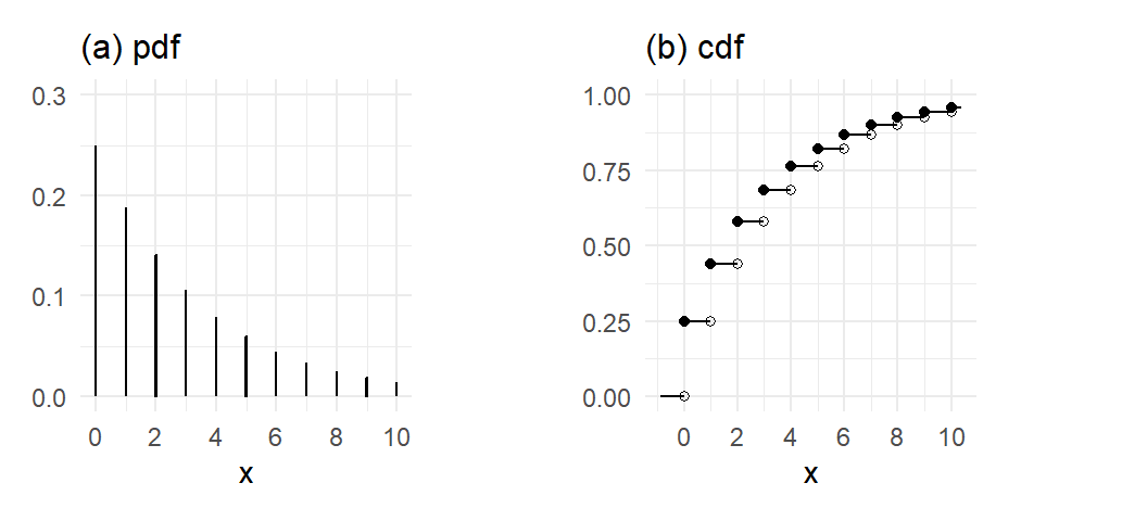
The probability density function of a discrete random variable is sometimes called a probability mass function and the cdf a cumulative probability mass function.
3.3.2 Uniform Distribution
Example 3.4 A random variable \(X\) has a \(\mathrm{Uniform}(0,1)\) distribution, written \(X \sim U(0,1)\), if its pdf is \[ f_X(x) = 1 \, , \, x \in [0,1]. \tag{3.13}\]
Whereas the probability density/mass function of a discrete random variable has the interpretation as \(f_X(x) = \mathrm{Pr}[X=x]\), this interpretation must be modified for continuous random variables. For continuous variables, the probability of obtaining an outcome between \(a\) and \(b\) is the area between the pdf and the \(x\)-axis from \(x=a\) to \(x=b\). That is, \[ \Pr[a \leq X \leq b] = \int_a^b f_X(u) \,du. \] For the Uniform (0,1) distribution, \(\mathrm{Pr}[a \leq X \leq b]\) is straightforward to compute. If \(X \sim U(0,1)\), then \(\mathrm{Pr}[0.1<X<0.3] = 0.2\), \(\mathrm{Pr}[X=0.5] = 0\), \(\Pr[0 \leq X \leq 1] = 1\), and so on. The cdf of the Uniform (0,1) random variable is \[ F_X(x) = \Pr[X \leq x] = \begin{cases} 0 \, , & x < 0 \\ x \, , & 0 \leq x \leq 1 \\ 1 \, , & x > 1. \end{cases} \, \]
## PDF
p1 <- ggplot() +
  geom_segment(data=data.frame(xstart=0, xend=1,ystart=1, yend=1),
               aes(x=xstart,y=ystart,xend=xend, yend=yend)) + ggtitle('(a) pdf') +
  xlim(-0.5,1.5) + ylim(0,1.2) + xlab("x") + ylab(NULL) + plot_theme
# CDF
p2 <- ggplot() +
  geom_segment(data=data.frame(xstart=c(-0.5,0,1), xend=c(0,1,1.5),
                               ystart=c(0,0,1), yend=c(0,1,1)),
  aes(x=xstart,y=ystart,xend=xend, yend=yend)) + ggtitle('(a) cdf') + xlim(-0.5,1.5) +
  ylim(0,1.2) + xlab("x") + ylab(NULL) + plot_theme
p1 | p2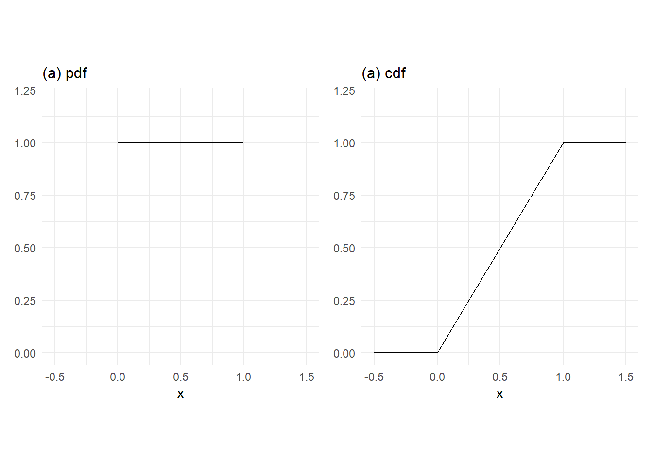
3.3.3 Mean, Variance and Other Moments
We have earlier introduced the mean and variance of discrete random variables with a finite number of outcomes. We extend these definitions to discrete random variables with countably infinite number of outcomes, and continuous random variables.
- If \(X\) has a finite number of possible outcomes \(x_1\),\(x_2\), …, \(x_n\) with probabilities \(p_1\),\(p_2\), …, \(p_n\) respectively, then \[ \begin{aligned} E[X] &= \sum_{i=1}^n x_i p_i \\ var[X] &= \sum_{i=1}^n (x_i - E[X])^2 p_i \end{aligned} \]
- If \(X\) has a infinitely countable number of possible outcomes \(x_1\),\(x_2\), … with probabilities \(p_1\),\(p_2\), … respectively, then \[ \begin{aligned} E[X] &= \sum_{i=1}^\infty x_i p_i \\ var[X] &= \sum_{i=1}^\infty (x_i - E[X])^2 p_i \end{aligned} \]
- If the possible values of \(X\) range over a continuum, and it has pdf \(f_X(x)\), then \[ \begin{aligned} E[X] &= \int xf_X(x) \, dx \\ var[X] &= \int (x-E[X])^2f_X(x) \, dx \end{aligned} \tag{3.14}\] where the integrals are over the range of possible values of \(X\). We can also write the variance definition as \[ \mathrm{var}[X] = \mathrm{E}[(X-\mathrm{E}[X])^2]. \tag{3.15}\] Sometimes easier to use \[ \mathrm{var}[X] = \mathrm{E}[X^2] - \mathrm{E}[X]^2. \tag{3.16}\] which you can derive from Eq. 3.15. The square root of the variance is called the standard deviation of \(X\).
Example 3.5
- If \(X \sim \mathrm{Bernoulli}(p)\), then \(E[X] = 1.p + 0.(1-p) = p\) and \(var[X] = p(1-p)\).
- If \(X \sim \mathrm{Geometric}(p)\), then \[ E[X] = \sum_{x=0}^\infty xp(1-p)^x = \frac{1-p}{p} \,\, \text{ (see exercises) }. \] Furthermore, \(E[X^2] = \sum_{x=0}^\infty x^2p(1-p)^x = \dfrac{(1-p)^2 + (1-p)}{p^2}\), therefore \[ var[X] = \frac{1-p}{p^2} \,\, \text{ (see exercises) }. \]
- If \(X \sim \mathrm{Uniform}(0,1)\), then \[ E[X] = \int_0^1 x \,dx = \frac{x^2}{2} \Big|_0^1 = \frac{1}{2}\,. \] Furthermore, \(E[X^2] = \int_0^1 x^2 \,dx = \dfrac{x^3}{3} \Big|_0^1 = \dfrac{1}{3}\), therefore \[ var[X] = \frac{1}{3} - \frac{1}{4} = \frac{1}{12}. \]
The important properties of the mean and variance continue to hold, i.e.,
- \(E[aX+b] = aE[X]+b\)
- \(var[aX+b] = a^2var[X]\)
where \(a\) and \(b\) are constants.
Besides the mean and variance, we occasionally refer to higher moments. The skewness coefficient of a random variable is defined to be \[ S = \frac{E[(X-E[X])^3]}{\sigma^3} \] where \(\sigma\) is the standard deviation of \(X\). It is used as a measure of symmetry. If a distribution is symmetric about the mean, then corresponding negative and positive deviations from mean receive the same weight, and retain their signs when raised to the third power. They therefore cancel out when summed or integrated, resulting in \(S=0\). E.g., the skewness coefficient of the normal distribution is zero.
The kurtosis of a random variable \(X\) is defined as \[ K = \frac{E[(X-E[X])^4]}{\sigma^4}. \] When raised to the fourth power, small deviation from means (\(<1\)) become very small and do not contribute to \(K\) whereas large deviations from mean contribute substantially. The kurtosis is therefore a measure of how “fat-tailed” a distribution is. It turns out that \(K=3\) for a normal-distributed random variable. A random variable with \(K>3\) is said to have excess kurtosis, or have a “fat-tailed” distribution.
3.3.4 The Normal Distribution
A random variable \(X\) has the normal distribution \(\mathrm{Normal}(\mu,\sigma^2)\) if it takes possible values over the entire real line, and its pdf is \[ f_{X}(x) = \frac{1}{\sigma \sqrt{2\pi}}\exp\left\{-\frac{(x - \mu)^2}{2\sigma^2}\right\} \, , \, x \in \mathbb{R}. \tag{3.17}\]
The pdf of the normal distribution has the familiar symmetric bell-shape, centered at \(\mu\), which is centered at \(\mu\). The variance is \(\sigma^{2}\). The normal distribution with mean 0 and variance 1 is called the standard normal distribution; it has no parameters, and has a special place in probability theory for reasons you will see in the next chapter.
Fig. 3.4 show 5 normal pdfs. The three centered at zero have mean zero. The thinner of these has variance 1/2, and the flatter, broader one as variance 4. The one in bold is the pdf of the standard normal. On either side are pdfs of normal variates with variance 1 and means -6 (left) and 6 (right).
x = seq(-10,10,0.01)
# dnorm(x,mu,sd) gives normal pdf at x with mean mu and standard deviation sd
fx_data = data.frame(x=x, fx_norm1=dnorm(x,0,1),
                          fx_norm2 = dnorm(x,0,sqrt(0.25)),
                          fx_norm3 = dnorm(x,0,sqrt(4)),
                          fx_norm4 = dnorm(x,-6,1),
                          fx_norm5 = dnorm(x,6,1))
p1 <- ggplot(data = fx_data) +
        geom_line(aes(x=x, y=fx_norm1), linewidth=1) +
        geom_line(aes(x=x, y=fx_norm2), linetype='dashed') +
        geom_line(aes(x=x, y=fx_norm3), linetype='dotted') +
        geom_line(aes(x=x, y=fx_norm4), color='blue', linewidth=0.75) +
        geom_line(aes(x=x, y=fx_norm5), color='magenta', linewidth=0.75) +
        annotate('text', -7.9, 0.4, label="Normal(-6,1)", color='blue', size=3) +
        annotate('text',  7.8, 0.4, label="Normal(6,1)", color='magenta', size=3) +
        annotate('text', 2.6, 0.25, label="Normal(0,1)", fontface='bold', size=3) +
        annotate('text', 2.3, 0.6, label="Normal(0,1/2)", size=3) +
        annotate('text', 4.3, 0.1, label="Normal(0,4)", size=3) +
        plot_theme + ylim(0,0.8) + ylab(NULL) + theme(aspect.ratio = 0.5)
p1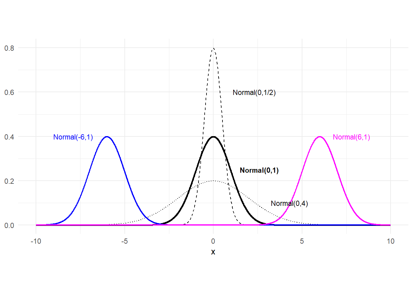
Substituting \(\mu=0\) and \(\sigma^2=1\) into Eq. 3.17 gives the pdf of the standard normal distribution, which is given the special notation \(\phi()\): \[ \phi(x) = \frac{1}{\sqrt{2\pi}}\exp\left\{-\frac{x^2}{2}\right\} \, , \, x \in \mathbb{R}. \tag{3.18}\] The normal distribution has the property that if \(X \sim \mathrm{Normal}(\mu, \sigma^2)\), then \[ aX+b \; \sim \; \mathrm{Normal}(a\mu+b, a^2 \sigma^2) \] The change in mean and variance will be true for all random variables; the important part here is that the distribution itself doesn’t change under the variable transformation. An important application of this result is: \[ \frac{X-\mu}{\sigma} \; \sim \; \mathrm{Normal}(0,1)\,. \] The cdf of the normal distribution is \[ F_{X}(x) = \Pr[X \leq x] = \int_{-\infty}^{\infty} \frac{1}{\sigma \sqrt{2\pi}}\exp\left\{-\frac{(x - \mu)^2}{2\sigma^2}\right\}\,dx \, , \, x \in \mathbb{R}. \tag{3.19}\] The normal cdf does not have a “closed form” expression (there isn’t a simple formula for it) but there are algorithms that can calculate it. The cdf of the standard normal is denoted \(\Phi(x)\).
x = seq(-4,4,0.01)
# pnorm(x,mu,sd) gives normal pdf at x with mean mu and standard deviation sd
fx_data = data.frame(x=x, fx_pnorm1 = pnorm(x,0,1))
p1 <- ggplot(data = fx_data) + geom_line(aes(x=x, y=fx_pnorm1), linewidth=0.75) +
        plot_theme + ylim(0,1.1) + ylab(NULL) + theme(aspect.ratio = 0.5)
p1
It is sometimes useful to express the pdf of a non-standard normal distribution in terms of the pdf and cdf of a standard normal. This is easily done given that linear transformations do not change the distributional form of a normal random variate. If \(X \sim N(\mu, \sigma^{2})\), then its cdf can be written as \[
F_X(x) = \Phi\left(\frac{x-\mu}{\sigma} \right)\,,
\] since \[
F_X(x) = \Pr (X \leq x) = \Pr\left(\frac{X-\mu}{\sigma} \leq \frac{x-\mu}{\sigma}\right) = \Phi\left( \frac{x-\mu}{\sigma} \right)\,.
\] Since the pdf is the derivative of the cdf, we have \[
f_X(x) = \frac{1}{\sigma} \phi\left( \frac{x-\mu}{\sigma} \right)\,.
\] The R function for the cdf of a normal variate with mean \(\mu\) and standard deviation \(\sigma\) is pnorm().
cat("pnorm(1,1,2) =", pnorm(1, mean=1, sd=2))
cat("\npnorm(2,1,2) =", pnorm(2, 1, 2))
cat("\npnorm(0,0,1) =", pnorm(0, 0, 1))
cat("\npnorm(-1.96,0,1) =", pnorm(-1.96, 0, 1))
cat("\npnorm(1.96,0,1) =", pnorm(1.96, 0, 1))
pnorm(1,1,2) = 0.5
pnorm(2,1,2) = 0.6914625
pnorm(0,0,1) = 0.5
pnorm(-1.96,0,1) = 0.0249979
pnorm(1.96,0,1) = 0.9750021To get the value of \(q\) such that \(X \leq q\), use qnorm():
cat("qnorm(0.025,0,1) =", qnorm(0.025, mean=0, sd=1)) qnorm(0.025,0,1) = -1.9599643.3.5 The Log-Normal Distribution
The log-normal distribution is sometimes used to describe the probabilistic behavior of stock prices. A random variable \(X\) has the log-normal distribution with distribution \(\mu\) and \(\sigma^2\) if its probability density function is \[ p_X(x) = \frac{1}{x\sigma \sqrt{2\pi}} \exp\left\{-\frac{(\ln x - \mu)^2}{2\sigma^2}\right\} \, , \, x \in (0,\infty). \tag{3.20}\] The log-normal distribution is so-called because if \(X \sim \mathrm{Lognormal}(\mu, \sigma^2)\), then \(Y = \ln X\) has the normal distribution \(\mathrm{Normal}(\mu,\sigma^2)\)
The log-normal cdf does not have ‘closed form’ expressions, but as with the normal distribution, that are computer algorithms that can compute the log-normal cdf to a good approximation.
x = seq(0.01,8,0.01)
fx_lnorm = dlnorm(x,1,1/2)
Fx_lnorm = plnorm(x,1,1/2)
p1 <- ggplot() +
        geom_line(data = data.frame(x,fx_lnorm), aes(x=x, y=fx_lnorm)) +
        plot_theme + ylim(0,0.4) + ylab(NULL) + ggtitle('(a) Lognormal pdf')
p2 <- ggplot() +
        geom_line(data = data.frame(x,Fx_lnorm), aes(x=x, y=Fx_lnorm)) +
        plot_theme + ylim(0,1) + ylab(NULL) + ggtitle('(b) Lognormal cdf')
(p1 | p2)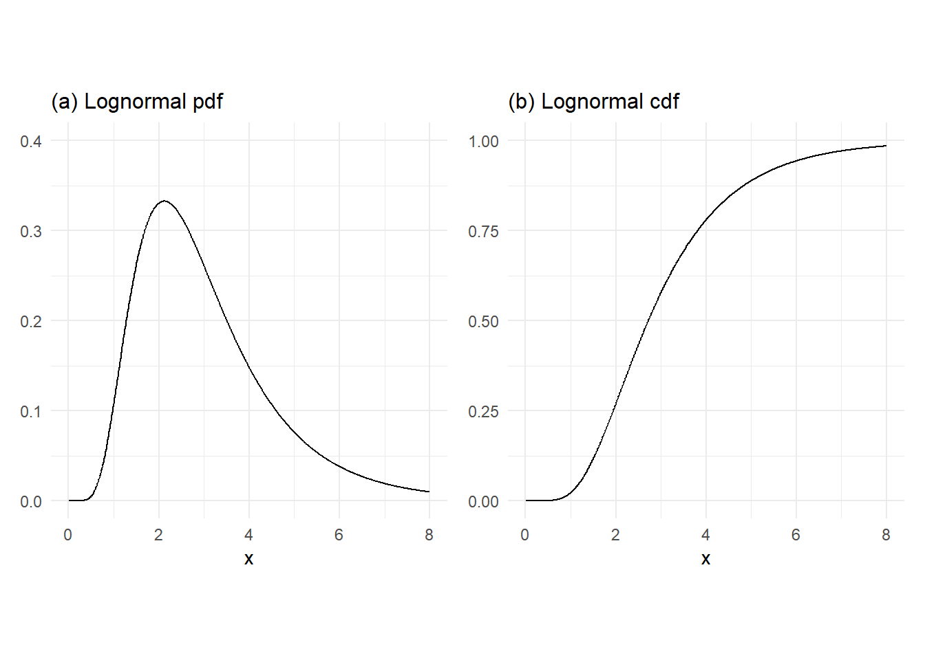
From the perspective of the validity of possible outcomes, the log-normal distribution, which takes possible values in \((0,\infty)\), is more appropriate than, say, the normal distribution, since prices cannot take negative values. However, there are many other distributions with possible outcomes restricted to \((0,\infty)\). Whether the log-normal distribution is the appropriate distribution for a given stock price is an empirical question.
- If \(X \sim \mathrm{Lognormal}(\mu,\sigma^2)\), then \[ \begin{aligned} E[X] &= \exp\left\{\mu + \frac{\sigma^2}{2}\right\} \\ var[X] &= [\exp(\sigma^2)-1]\exp(2\mu+\sigma^2) \end{aligned} \]
3.3.6 The Chi-squared, Student-t, and F Distributions
We mention three univariate distributions that are related to the normal distribution. We will not need to use the expression of the pdf or cdf of these distributions, but you will need to know the properties that we list here.
3.3.6.1 Chi-square distribution
If \(X \sim N(0,1)\), then \(X^2\) has the “Chi-squared distribution with one degree of freedom”. If \(X_1,X_2,\dots,X_k\) are independent standard normal variates, then \(\sum_{i=1}^k X_i^2\) is Chi-squared distribution with \(k\) degrees of freedom, denoted \(\chi^2_{(k)}\). If \(X \sim \chi^2_{(k)}\), then \(E[X]=k\) and \(var[X]=2k\).
x = seq(0.05, 30, 0.01)
df_chi <- data.frame(x = x, fx_chi1 = dchisq(x,1), fx_chi5 = dchisq(x,5),
                     fx_chi10 = dchisq(x,10), fx_chi20 = dchisq(x,20))
p1 <- ggplot(data = df_chi) +
        geom_line(aes(x=x, y=fx_chi1), linewidth=0.5) +
        geom_line(aes(x=x, y=fx_chi5), linewidth=0.5) +
        geom_line(aes(x=x, y=fx_chi10), linewidth=0.5) +
        geom_line(aes(x=x, y=fx_chi20), linewidth=0.5) +
        annotate('text',  2.3, 0.23, label=TeX("$\\chi^{2}$(1)")) +
        annotate('text',  5, 0.17, label=TeX("$\\chi^{2}$(5)")) +
        annotate('text',  10, 0.12, label=TeX("$\\chi^{2}$(10)")) +
        annotate('text',  21, 0.08, label=TeX("$\\chi^{2}$(20)")) +
        plot_theme + ylim(0,0.25) + ylab(NULL) + theme(aspect.ratio = 0.5)
p1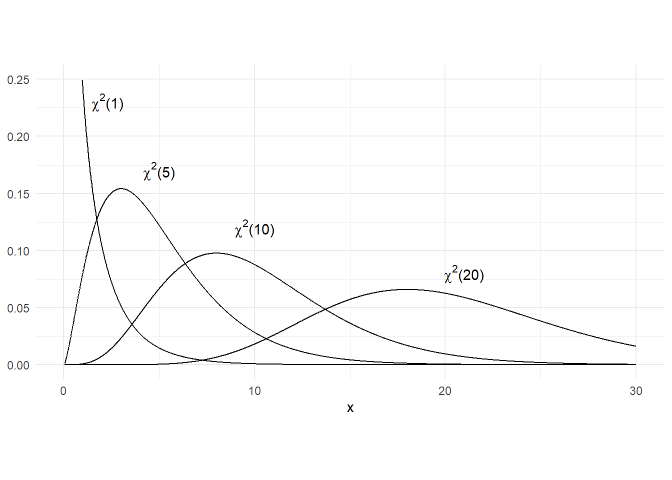
3.3.6.2 Student-t distribution
If \(X\) and \(W\) are independent variables with \(X \sim N(0,1)\) and \(W \sim \chi^2(k)\), then \[ \frac{X}{\sqrt{W / k}} \sim \mathrm{t}_{(v)} \] where \(\mathrm{t}_{(v)}\) denotes the “Student-t distribution with \(v\) degrees of freedom”. A student-t random variate has zero mean, and variance \(\frac{v}{v-2}\) (the variance does not exist unless \(v>2\)). The Student-t pdf is similar to that of the standand normal pdf in that it is symmetrically bell-shaped and centered about zero. However, it has fatter tails than a normal distribution (its kurtosis is always greater than 3). This means that a Student-t random variable has greater probability of extreme realizations than a comparable normal variate. The Student-t pdf has the property that it converges to the standard normal pdf as \(v \rightarrow \infty\). Fig. 3.8 shows the student-t pdf with degree-of-freedom parameter v=1, 5, 10, and 20, and also the pdf of the standard normal. The t(1) and t(5) distributions are indicated, with the t(10) and t(20) distributions “between” the t(5) and the Normal(0,1) pdf.
x = seq(-5, 5, 0.01)
df_t <- data.frame(x = x, fx_t1 = dt(x,1), fx_t5 = dt(x,5), fx_t10 = dt(x,10),
                   fx_t20 = dt(x,20), fx_norm = dnorm(x,0,1))
p1 <- ggplot(data = df_t) +
        geom_line(aes(x=x, y=fx_t1), linewidth=0.5) +
        geom_line(aes(x=x, y=fx_t5), linewidth=0.5) +
        geom_line(aes(x=x, y=fx_t10), linewidth=0.5) +
        geom_line(aes(x=x, y=fx_t20), linewidth=0.5) +
        geom_line(aes(x=x, y=fx_norm), linewidth=0.6, color="magenta") +
        annotate('text',  0.8, 0.13, label="t(1)") +
        annotate('text',  0.08, 0.34, label="t(5)") +
        annotate('text',  0.89, 0.38, label="N(0,1)", color="magenta") +
        plot_theme + ylim(0, 0.42) + ylab(NULL) +
        theme(aspect.ratio = 0.5)
p1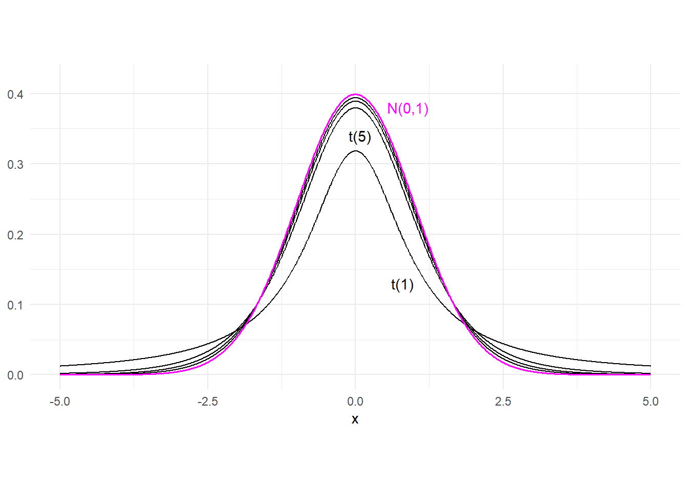
The following table compares the tail probabilities of the normal and the t distribution.
norm_vs_t_tail <- cbind(
                    pnorm(c(-2.57, -1.96, -1.64)),
                    pt(c(-2.57, -1.96, -1.64), 1),
                    pt(c(-2.57, -1.96, -1.64), 5),
                    pt(c(-2.57, -1.96, -1.64), 10),
                    pt(c(-2.57, -1.96, -1.64), 20),
                    pt(c(-2.57, -1.96, -1.64), 30))
colnames(norm_vs_t_tail) <- c("N(0,1)", "t(1)", "t(5)", "t(10)", "t(20)", "t(30)")
rownames(norm_vs_t_tail) <- c("P[X<-2.57]", "P[X<-1.96]", "P[X<-1.64]")
round(norm_vs_t_tail, 4)
N(0,1) t(1) t(5) t(10) t(20) t(30)
P[X<-2.57] 0.0051 0.1181 0.0250 0.0139 0.0091 0.0077
P[X<-1.96] 0.0250 0.1502 0.0536 0.0392 0.0320 0.0297
P[X<-1.64] 0.0505 0.1743 0.0810 0.0660 0.0583 0.05573.3.6.3 F distribution
If \(W_1\) and \(W_2\) are independent chi-squared random variables with degrees of freedom \(v_1\) and \(v_2\) respectively, then \[ \frac{W_1 / v_1}{W_2 / v_2} \sim F_{(v_1,v_2)} \] where \(F_{(v_1,v_2)}\) denotes the “F distribution with \(v_1\) and \(v_2\) degrees of freedom”. If \(X \sim F_{(v_1,v_2)}\), then \[ \begin{gathered} E[X] = \frac{v_2}{v_2-2} \\ var[X] = 2\left(\frac{v_2}{v_2-2}\right)^2\frac{v_1+v_2-2}{v_1(v_2-4)}\;. \end{gathered} \]
The F-distribution is also related to the t- and chi-squared distributions in that
- If \(X \sim t_{(v)}\), then \(X^2 \sim F_{(1,v)}\),
- If \(X \sim F_{(v_1,v_2)}\), then the pdf of \(v_1X\) converges to the \(\chi^2(v_1)\) pdf as \(v_2 \rightarrow \infty\).
Fig. 3.9 shows the \(F_{(3,10)}\) pdf.
x <- seq(0,5,0.01)
Fpdf <- df(x, df1=3, df2=20)
dat2 <- data.frame(x , Fpdf)
p1 <- ggplot(data = dat2) +
      geom_line(aes(x=x, y = Fpdf), colour="black") +
      ggtitle(TeX("$F_{(3,20)}$ pdf")) + ylab(NULL) + theme_minimal() +
      theme(aspect.ratio = 0.5)
p1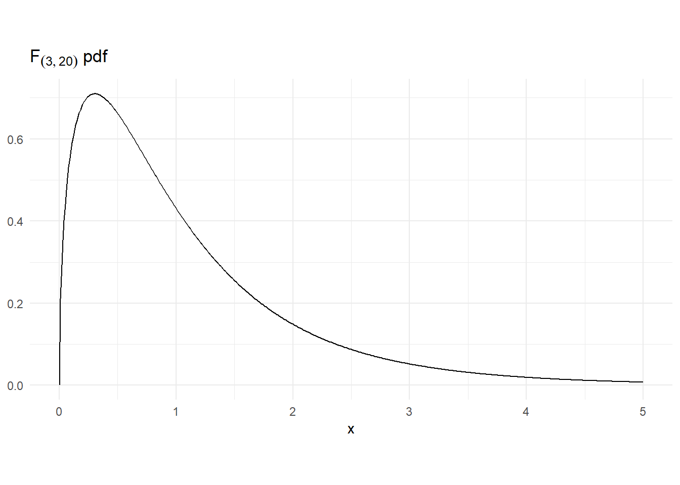
3.3.7 The Bivariate Normal Distribution
Two random variables \(X\) and \(Y\) have the bivariate normal distribution if their joint pdf have the form \[ f_{X,Y}(x,y) = \frac{1}{2\pi\sigma_x\sigma_y\sqrt{1-\rho_{xy}^2}} \exp\left\{ -\frac{1}{2}\frac{\widetilde{x}^2 - 2\rho_{xy}\widetilde{x} \widetilde{y} + \widetilde{y}^2} {1-\rho_{xy}^2} \right\} \tag{3.21}\] where \(\widetilde{x}=\dfrac{x-\mu_x}{\sigma_x}\) and \(\widetilde{y}=\dfrac{y-\mu_y}{\sigma_y}\). The bivariate normal distribution has five parameters, with the following interpretation:
- \(\mu_x\) : unconditional mean of \(X\),
- \(\mu_y\) : unconditional mean of \(Y\),
- \(\sigma_x^2\) : unconditional variance of \(X\),
- \(\sigma_y^2\) : unconditional variance of \(Y\), and
- \(\rho_{xy}\) : correlation coefficient of \(X\) and \(Y\), i.e., \(\rho = \dfrac{\sigma_{xy}}{\sigma_x\sigma_y}\) where \(\sigma_{xy} = cov[X,Y]\).
We write \((X,Y) \sim \mathrm{Normal}_2(\mu_x, \mu_y, \sigma_x^2, \sigma_y^2, \rho_{xy})\)
Contour plots are helpful for visualizing bivariate normal distributions. We show the contour plots of a bivariate normal distribution with \[ (\mu_x, \mu_y, \sigma_x^2, \sigma_y^2, \rho) = (1, 0, 1, 2, 0.9). \] in Fig. 3.10(a). Alternatively, one can look at the 3-d plot of the bivariate pdf in Fig. 3.10(b).
x <- seq(-3,5,0.2)
y <- seq(-4,4,0.2)
mesh_xy <- expand.grid(x,y)
binorm1 <- function(mesh_xy, mu1, mu2, sg1, sg2, rho){
  r <- (2*pi*sg1*sg2*sqrt(1-rho^2))^(-1)*exp(-1/(2*(1-rho^2))*
        (((mesh_xy[,1]-mu1)/sg1)^2 - 2*rho*(mesh_xy[,1]-mu1)*(mesh_xy[,2]-mu2)/sg1/sg2
           + ((mesh_xy[,2]-mu2)/sg2)^2))
}
binorm2 <- function(x,y, mu1, mu2, sg1, sg2, rho){
  r <- (2*pi*sg1*sg2*sqrt(1-rho^2))^(-1)*exp(-1/(2*(1-rho^2))*
        (((x-mu1)/sg1)^2 - 2*rho*(x-mu1)*(y-mu2)/sg1/sg2 + ((y-mu2)/sg2)^2))
}
par(mfrow=c(1,2))
mu1 <- 1; mu2 <- 0; sg1 <- 1; sg2 <- sqrt(2); rho = 0.7
par(mar=c(2,1.5,1.5,1.5))  # Contour
f_xy <- binorm1(mesh_xy, mu1, mu2, sg1, sg2, rho)
f_xy <- matrix(f_xy, byrow=FALSE, nrow=length(x))
p1 <- contour(x,y,f_xy,nlevels=12, xlab="", ylab="", main="(a) Contour Plot",
              cex.lab=0.6, cex.axis=0.6, cex.main=0.6)
title(ylab="y", line=-1, cex.lab=0.6)
title(xlab="x", line=-1, cex.lab=0.6)
par(mar=c(0,1,0,0)) # 3-d
z <- outer(x,y,binorm2, mu1, mu2, sg1, sg2, rho)
p2 <- persp(x,y,z,theta=20, phi=30, r=10, expand=0.8, col="lightblue",
      ltheta=0, shade=0.75,ticktype="detailed", xlab="x", ylab="y", zlab="",
      cex.lab=0.6, cex.axis=0.6)
title(main="(b) 3-d Plot", cex.main=0.6, line=-1)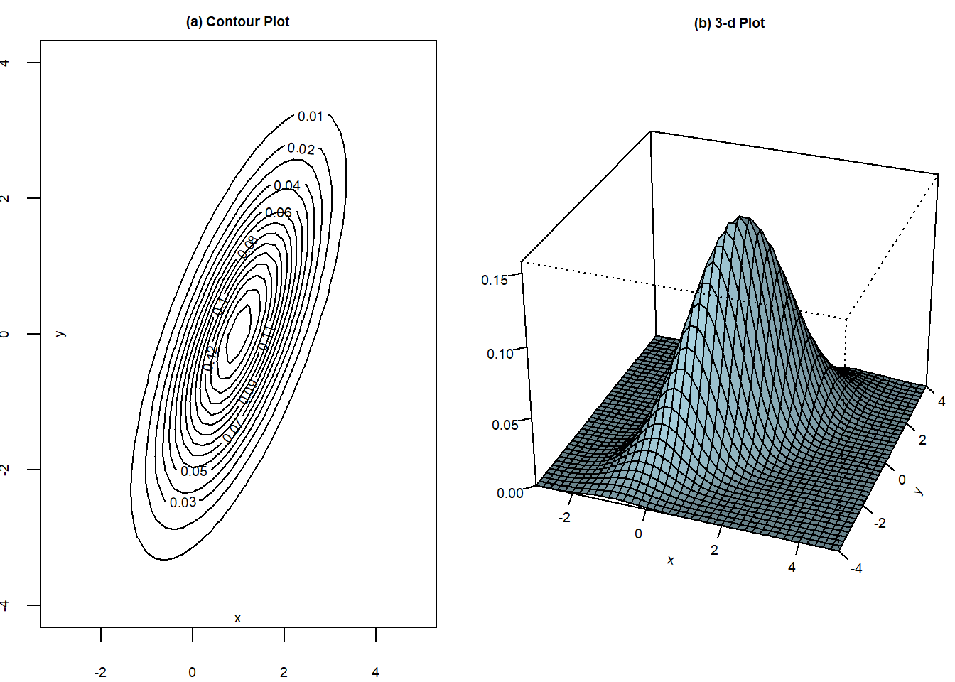
The marginal and conditional distributions of a bivariate normal random variables are also normal. To see this, we “complete the square” on \(\widetilde{x}^2 - 2\rho_{xy}\widetilde{x} \widetilde{y} + \widetilde{y}^2\) to get \[ \begin{aligned} \widetilde{x}^2 - 2\rho_{xy}\widetilde{x} \widetilde{y} + \widetilde{y}^2 & = (\widetilde{x} - \rho_{xy} \widetilde{y})^2 + (1 - \rho_{xy}^2) \widetilde{y}^2 \\ & = \left[\frac{x - \mu_x}{\sigma_x} - \frac{\sigma_{xy}}{\sigma_x\sigma_y}\frac{y-\mu_y}{\sigma_y} \right]^2 + (1 - \rho_{xy}^2) \left( \frac{y-\mu_y}{\sigma_y} \right)^2 \\ & = \frac{1}{\sigma_x^2}\left[x - \mu_x - \frac{\sigma_{xy}}{\sigma_y^2}(y-\mu_y) \right]^2 + (1 - \rho_{xy}^2) \left( \frac{y-\mu_y}{\sigma_y} \right)^2 \\ & = \frac{1}{\sigma_x^2}\left[x - (\alpha + \beta y) \right]^2 + (1 - \rho_{xy}^2) \left( \frac{y-\mu_y}{\sigma_y} \right)^2 \end{aligned} \] where \(\alpha = \mu_x - \beta \mu_y\) and \(\beta = \dfrac{\sigma_{xy}}{\sigma_y^2}\). Then the pdf can be written as \[ \begin{aligned} &f_{X,Y}(x,y) \\ &= \frac{1}{2\pi\sigma_x\sigma_y\sqrt{1-\rho_{xy}^2}} \exp\left\{-\frac{1}{2} \frac{1}{1-\rho_{xy}^2}(\widetilde{x}^2 - 2\rho_{xy}\widetilde{x} \widetilde{y} + \widetilde{y}^2) \right\} \\ &= \frac{1}{2\pi\sigma_x\sigma_y\sqrt{1-\rho_{xy}^2}} \times \exp\left\{-\frac{1}{2} \frac{1}{1-\rho_{xy}^2} \left[ \frac{1}{\sigma_x^2}\left[x - (\alpha + \beta y) \right]^2 + (1 - \rho_{xy}^2) \left( \frac{y-\mu_y}{\sigma_y} \right)^2 \right] \right\} \\ &=\underbrace{ \frac{1}{\sqrt{2\pi}\sqrt{\sigma_x^2(1-\rho_{xy}^2)}} \exp\left\{-\frac{1}{2} \frac{\left[x - (\alpha + \beta y) \right]^2}{\sigma_x^2(1-\rho_{xy}^2)} \right\} }_{A} \times \underbrace{ \frac{1}{\sqrt{2\pi}\sigma_y} \exp\left\{ -\frac{1}{2} \left( \frac{y-\mu_y}{\sigma_y} \right)^2 \right\} }_{B} \end{aligned} \] If we compare expressions \(A\) and \(B\) with the expression for the Normal pdf, we see that \(B\) is a normal pdf \(f_Y(y)\) with mean \(\mu_y\) and variance \(\sigma_y\), and if we take \(y\) as fixed, then \(A\) is a (conditional) normal pdf \(f_{X|Y}(x|y)\) with mean \(\alpha + \beta y\) and variance \(\sigma_x^2 - \sigma_{xy}/\sigma_y^2\). That is, if \(X\) and \(Y\) have the bivariate normal distribution Eq. 3.21, then
- the marginal distribution of \(Y\) is \(\mathrm{Normal}(\mu_y, \sigma_y^2)\),
- the conditional distribution of \(X\) given \(Y\) is \(\mathrm{Normal}(\mu_{x|y}, \sigma_{x|y})\) where
\[ \begin{aligned} \mu_{x|y} &= \mu_x + \frac{\sigma_{xy}}{\sigma_y^2}(y-\mu_y), \\ \sigma_{x|y} &= \sigma_x^2 - \dfrac{\sigma_{xy}}{\sigma_y^2}. \end{aligned} \] The conditional mean can be written as \(\mu_{x|y} = \alpha_x + \beta_x y\) where \(\alpha_x = \mu_x - \beta_x \mu_y\) and \(\beta_x = \dfrac{\sigma_{xy}}{\sigma_y^2}\).
Similarly,
- the marginal distribution of \(X\) is \(\mathrm{Normal}(\mu_x, \sigma_x^2)\),
- the conditional distribution of \(Y\) given \(X\) is \(\mathrm{Normal}(\mu_{y|x}, \sigma_{y|x})\) where \[ \begin{aligned} \mu_{y|x} &= \mu_y + \frac{\sigma_{xy}}{\sigma_x^2}(x-\mu_x), \\ \sigma_{y|x} &= \sigma_y^2 - \dfrac{\sigma_{xy}}{\sigma_x^2}. \end{aligned} \]
The conditional mean can be written as \(\mu_{y|x} = \alpha_y + \beta_y x\) where \(\alpha_y = \mu_y - \beta_y \mu_x\) and \(\beta_y = \dfrac{\sigma_{xy}}{\sigma_x^2}\).
It follows immediately from the decomposition of the bivariate normal pdf that \(X\) and \(Y\) are independent if they are bivariate normal and uncorrelated (see exercises). It can also be shown that if \(X\) and \(Y\) are bivariate normal, then
- \(aX + bY \sim \text{Normal}(a\mu_x + b\mu_y \, , \, a^2\sigma_x^2 + b^2\sigma_y^2 + 2ab\sigma_{xy})\).
We omit the proof of this last result.
3.3.8 Exercises
Exercise 3.11 Use the fact that \[ \sum_{j=0}^\infty jr^j = \frac{r}{(1-r)^2} \,\, \text{ and } \sum_{j=0}^\infty j^2r^j = \frac{r^2 + r}{(1-r)^3} \] to derive the mean and variance of the Geometric distribution.
Exercise 3.12 Show that \(X\) and \(Y\) are independent if they are bivariate normal and uncorrelated. Hint: show that \(f_{X,Y}(x,y) = f_{Y}(y)f_X(x)\) when \(\rho_{xy}=0\).
Exercise 3.13 The function pnorm(), when evaluated at \(x\), returns the CDF of the normal pdf at \(x\), i.e., it returns the probability \(\Pr[X\leq x]\). The quantile function qnorm(), when evaluated at probability \(p\), returns the value of \(x\) for which \(\Pr[X\leq x] = p\). For example:
pnorm(0, mean=0, sd=1) # Pr[X <= 0] for X~N(0,1)[1] 0.5qnorm(0.5, mean=0, sd=1) # c such that Pr[X<=c]=0.5 when X~N(0,1)[1] 0The corresponding functions for the t, chi-sq, and F distributions are pt(x,df) and qt(p, df), pchisq(x,df) and qchisq(p,df), and pf(x,df1,df2) and qf(p,df1, df2) respectively. Find:
\(\Pr[X\leq -2.5]\) when \(X\sim N(0,1)\)
\(\Pr[X\leq -2.5]\) when \(X\sim t_{(5)}\)
\(c\) such that \(\Pr[X > c] = 0.05\) when \(X\sim \chi^2_{(5)}\).
\(\Pr[-1.96 \leq X \leq 1.96]\) when \(X\sim N(0,1)\)
\(c\) such that \(\Pr[-c \leq X \leq c] = 0.95\) when \(X\sim N(0,1)\)
\(c\) such that \(\Pr[-c \leq X \leq c] = 0.95\) when \(X \sim t_{(12)}\)
\(c\) such that \(\Pr[-c \leq X \leq c] = 0.95\) when \(X \sim t_{(100)}\)
\(c\) such that \(\Pr[X > c] = 0.05\) when \(X\sim F_{(5,8)}\).
\(5c\) such that \(\Pr[X > c] = 0.05\) when \(X\sim F_{(5,80)}\).
\(5c\) such that \(\Pr[X > c] = 0.05\) when \(X\sim F_{(5,8000)}\).
3.4 Prediction
The prediction problem is, roughly: given the realization of \(X\), what is \(Y\)? In other words, if I tell you that the realization of \(X\) is \(x\) (this is your “information set”), what can you tell me about \(Y\)? Often what is wanted is some estimate of what \(Y\) will turn out to be, e.g., what is the price of a house in a particular city given that it is in such-and-such location, is 15 years old, and has four rooms? The desired answer is some value, such as, 1.8 million dollars. This is a “point prediction”. Sometimes we want other types of prediction, such as “what is the probability that inflation will exceed 5 percent over the next quarter?” This is a “probabilistic forecast”, and the information set would presumably be current and past realizations of all variables that the forecaster deems relevant for inflation.
Suppose what we want is a point prediction of \(Y\) given knowledge that \(X = x\), and suppose we have a squared error loss function, meaning that if our prediction is \(\hat{y}(x)\) and the realization of \(Y\) turns out to be \(y\), then the cost of prediction error is \((y - \hat{y}(x))^{2}\). Suppose the prediction is made to minimize expected loss, i.e., we choose \(\hat{y}(x)\) to minimize the (Conditional) Mean Squared Prediction Error (MSPE) \[ MSPE(Y|X=x) = E[(Y-\hat{y}(x))^{2} | X = x]\,. \tag{3.22}\] The question is how to choose \(\hat{y}(x)\).
Unsurprisingly, the optimal prediction (the prediction that minimizes Eq. 3.22) is the conditional mean \(E[Y|X=x]\), as we now show. Write the MSPE as \[ \begin{aligned} MSPE(Y|X=x) &= E[(Y-E[Y|X=x] + E[Y|X=x] - \hat{y}(x))^{2} | X = x] \\[1ex] &= E[(Y-E[Y|X=x])^{2}|X=x] + E[(E[Y|X=x] - \hat{y}(x))^{2} | X = x] \; + \\[0.5ex] &\qquad \qquad \qquad 2 E[(Y-E[Y|X=x])(E[Y|X=x] - \hat{y}(x)) | X = x] \\[1ex] &= E[(Y-E[Y|X=x])^{2}| X=x] + (E[Y|X=x] - \hat{y}(x))^{2}\,. \end{aligned} \] The last equality holds because the second term in the RHS of the second line is fixed given \(X=x\), and the third term is zero.2 The first term on the RHS of the last line does not depend on the prediction, and since the second term is non-negative, the prediction that minimizes \(MSPE(Y|X=x)\) is the conditional expectation \(E[Y|X=x]\). Since \(E[Y|X]\) minimizes conditional \(MSPE\) for all possible values \(x\) of \(X\), it also minimizes the unconditional MSPE.
Of course in practice we do not know the conditional distribution \(E[Y|X=x]\), and will have to estimate it from previously taken observations of \(Y\) and \(X\).