We cover four topics in matrix algebra: matrix rank, diagonalization of matrices, differentiation of matrix forms, and vectors and matrices of random variables.
8.1 Rank
8.1.1 A Geometric Viewpoint
We consider vectors and matrices from a geometric perspective, leading up to the concept of the rank of a matrix. We view a 2-dimensional vector \[
v_1 = \begin{bmatrix} x_1 \\ y_1 \end{bmatrix}
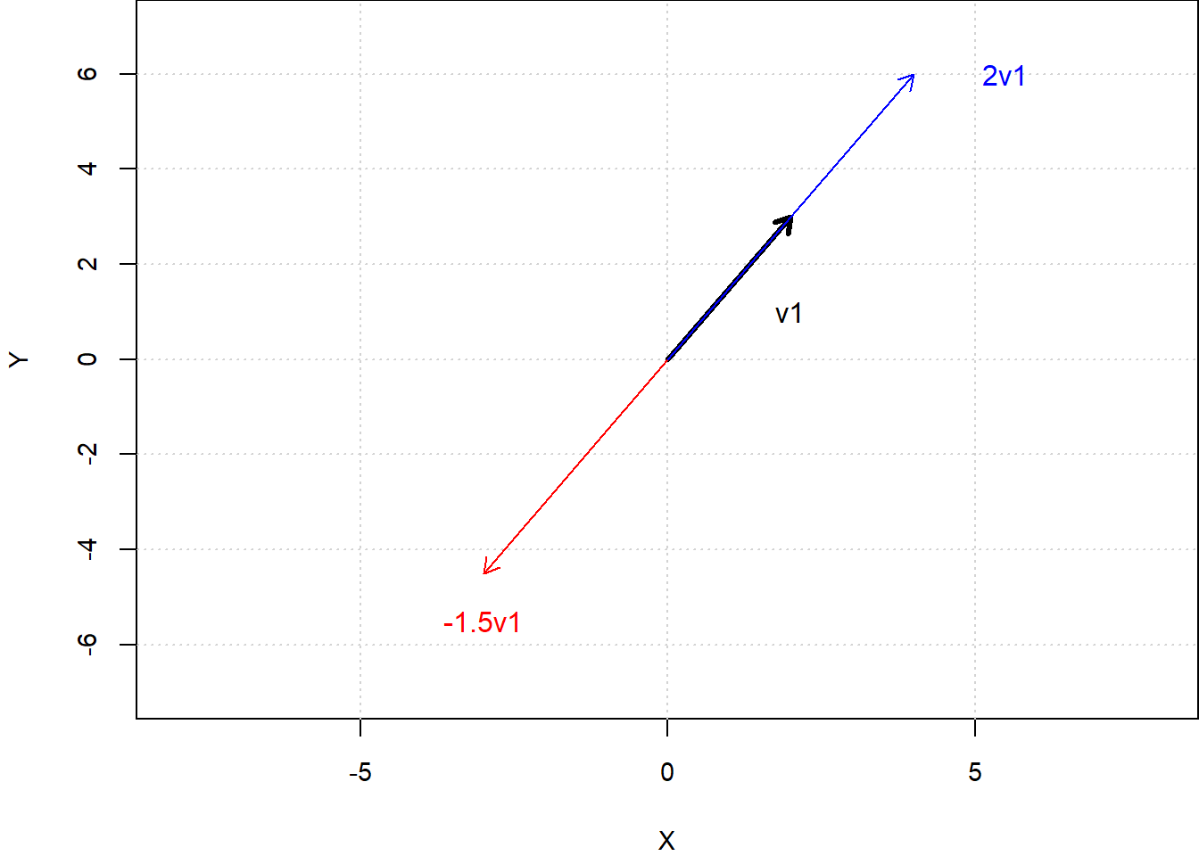
\] as an arrow from the origin to the point \((x_1,y_1)\). For the moment, we focus on column vectors. Fig. 8.1 shows three vectors, where \(v_{2}\) and \(v_{3}\) are scalar multiples of \(v_{1}\). \[
v_1 = \begin{bmatrix} 2 \\ 3 \end{bmatrix},
v_2 = -1.5\begin{bmatrix} 2 \\ 3 \end{bmatrix},
v_3 = 2\begin{bmatrix} 2 \\ 3 \end{bmatrix}.
\]
Multiplying a non-zero vector by a scalar changes its length (stretch or shrink). If the scalar is negative, the vector direction is reversed. Other than possibly reversing direction, there is no rotation. If we take the set of all vectors of the form \(cv_{1}\), \(c\in\mathbb{R}\), we get a straight line, which we can think of as a “one-dimensional space” in the two dimensional space made up of all two-dimensional vectors.
Now view a \((2 \times 2)\) matrix as a collection of two column vectors \[
A =
\begin{bmatrix}
v_{11} & v_{12} \\ v_{21} & v_{22}
\end{bmatrix}
=
\begin{bmatrix}
\begin{bmatrix} v_{11} \\ v_{21} \end{bmatrix}
& \begin{bmatrix} v_{12} \\ v_{22} \end{bmatrix}
\end{bmatrix}
=
\begin{bmatrix}
v_1 & v_2
\end{bmatrix}\,.
\] Consider linear combinations of the two vectors \(v_1\) and \(v_2\): \[
c_1 v_1 + c_2 v_2
=
\begin{bmatrix}
v_1 & v_2
\end{bmatrix}
\begin{bmatrix}
c_1 \\ c_2
\end{bmatrix}
= Ac\,.
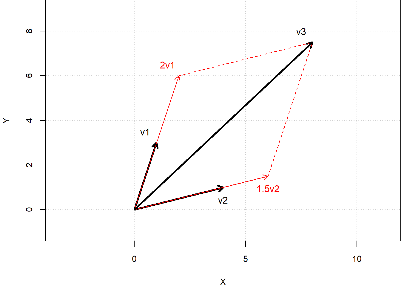
\] The result is a third vector that is a diagonal of the parallelogram formed by \(c_1v_1\) and \(c_2v_2\). This is illustrated in Fig. 8.2 for \(c_1 = 2\) and \(c_2 = 1.5\). \[
v_1 = \begin{bmatrix} 1 \\ 3 \end{bmatrix},
v_2 = \begin{bmatrix} 4 \\ 1 \end{bmatrix},
v_3 = 2v_1 + 1.5v_2 = \begin{bmatrix} 8 \\ 7.5 \end{bmatrix}.
\]
Now we consider, given two vectors \(v_1\) and \(v_2\), the set of all linear combinations of the form \(c_1v_1 + c_2v_2\), where \(c_1 \in \mathbb{R}\) and \(c_2 \in \mathbb{R}\). We consider in particular the following cases:
Case 1: \(v_1\) and \(v_2\) are non-zero vectors, and it is not the case that \(v_1 = bv_2\). The example in Fig. 8.2 illustrates this case. In such situations, the set of all linear combinations \(c_1v_1 + c_2v_2\) fills the entire 2-d space. Put differently, given any vector in the \(x\)-\(y\) plane, you can find \(c_1\) and \(c_2\) such that that vector is equal to \(c_1v_1 + c_2v_2\). We say \(v_1\) and \(v_2\)spans the entire 2-d space, and that the matrix \(A = \begin{bmatrix} v_1 & v_2 \end{bmatrix}\) has column rank two. Since the column rank of \(A\) is equal to the number of columns in \(A\), we also say \(A\) has full column rank.
Case 2: \(v_1 = bv_2\) (i.e., \(v_1\) and \(v_2\) lie on the same line) or if one of the vectors is a zero vector and the other is not. In this case, then the set of all possible linear combinations \(c_1v_1 + c_2v_2\) will be the line coincident with \(v_1\) and \(v_2\), or the line coincident with the non-zero vector. The vectors \(v_1\) and \(v_2\) do not span the entire (two-dimensional) space, but span only a (one-dimensional) line. The matrix \(A = \begin{bmatrix} v_1 & v_2 \end{bmatrix}\) will take the form \[
A =
\begin{bmatrix}
v_{11} & bv_{11} \\ v_{21} & bv_{21}
\end{bmatrix},
\begin{bmatrix}
v_{11} & 0 \\ v_{21} & 0
\end{bmatrix}
\text{ or }
\begin{bmatrix}
0 & v_{12} \\ 0 & v_{22}
\end{bmatrix}
\] We say the matrix \(A\) has column rank one.
Case 3: \(v_1 = v_2 = 0\). In this case, all linear combinations \(c_1v_1 + c_2v_2\) result in the zero vector. We say that the matrix \[
A = \begin{bmatrix} v_1 & v_2 \end{bmatrix}
=
\begin{bmatrix}
0 & 0 \\ 0 & 0
\end{bmatrix}
\] has column rank 0.
Notice that in cases 2 and 3, we have \[
c_1v_1 + c_2v_2 = 0 \text{ for some } (c_1, c_2) \neq (0,0),
\text{ or }
Ac = 0 \text{ for some } c \neq 0
\tag{8.1}\] whereas in case 1 \[
c_1v_1 + c_2v_2 \neq 0 \text{ for all } (c_1, c_2) \neq (0,0),
\text{ i.e., }
Ac \neq 0 \text{ for all } c \neq 0\,.
\tag{8.2}\] We say the vectors are linearly dependent if (8.1) holds, and linearly independent if (8.2) holds.
We can view a \((2 \times m)\) matrix, \(m>2\), as a collection of \(m\) 2-d vectors. These are vectors ‘living’ in 2-d space. Again, we consider the set of all linear combinations of the form \[
c_1v_1 + c_2v_2 + \dots + c_mv_m\,.
\] Depending on the values of the vectors, the vectors might span the entire 2-d space, or only a single (1-d) line, or just the origin if the vectors are all zero-vectors. However, 2-d vectors cannot span a three (or more) dimensional space, no matter how many of them there are. In other words, a \((2 \times m)\) matrix \(A\), with \(m>2\), may have column rank 2, 1, or 0, but cannot have column rank greater than 2. Put yet another way, a set of three or more 2-d vectors must be linearly dependent. We will be able to write each one as some combination of the others.
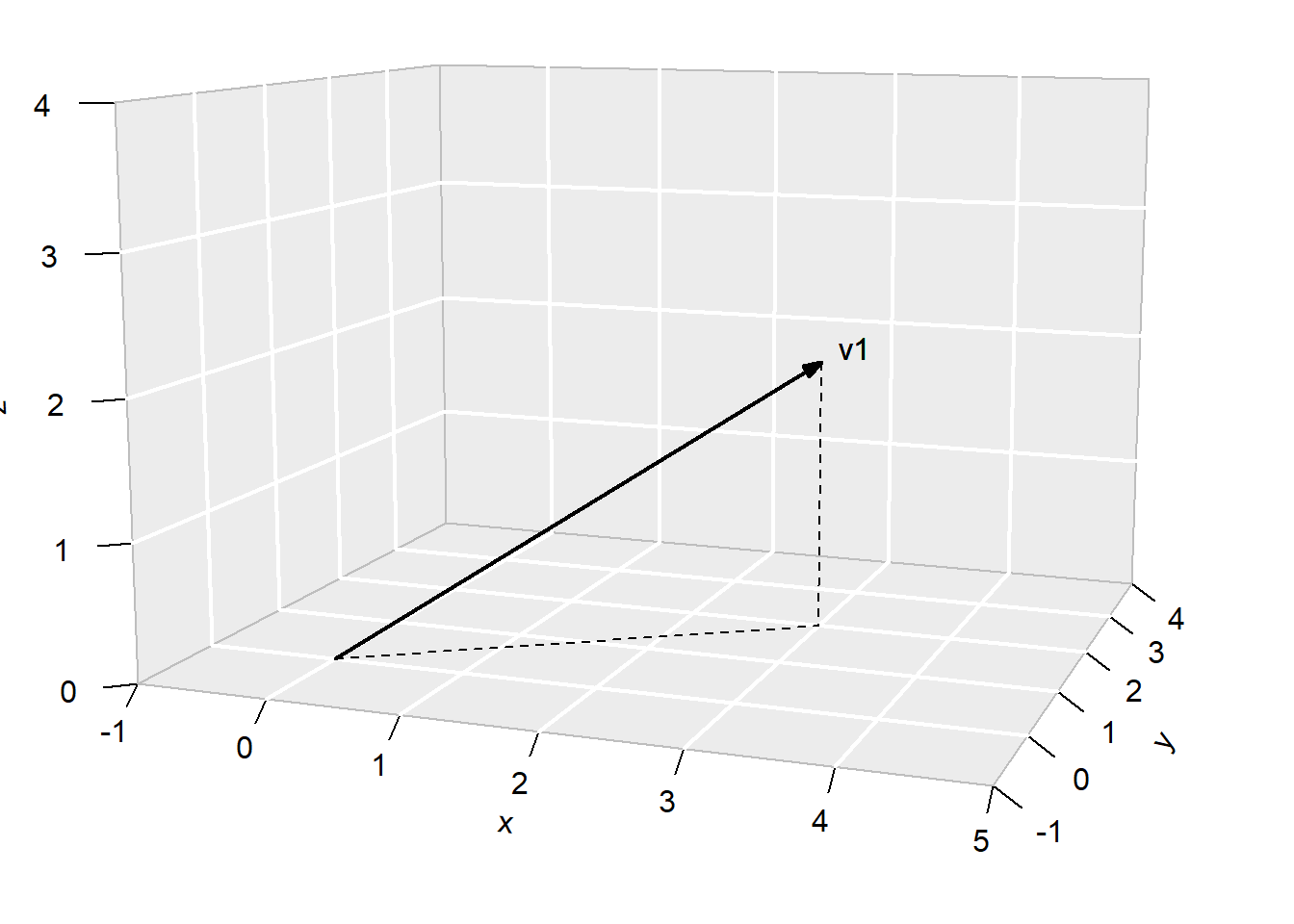
We view a 3-dimensional vector \[
v_1 = \begin{bmatrix} x_1 \\ y_1 \\ z_1 \end{bmatrix}
\] as an arrow in a three-dimensional cartesian space from the origin to the point \((x_1,y_1, z_1)\). The diagram below illustrates1 the vector \[
v_1 = \begin{bmatrix} 3 \\ 2 \\ 2 \end{bmatrix}.
\]
Figure 8.3: A 3-d vector.
Multiplying a vector by a scalar changes its length, but not the direction, except if the scalar is negative, in which case the vector direction is flipped. All vectors \(cv_1\) for any scalar \(c\) will lie on a single line.
View a \((3 \times 2)\) matrix as a collection of two 3-d column vectors \[
A =
\begin{bmatrix}
v_{11} & v_{12} \\ v_{21} & v_{22} \\ v_{31} & v_{32}
\end{bmatrix}
=
\begin{bmatrix}
\begin{bmatrix} v_{11} \\ v_{21} \\ v_{31} \end{bmatrix}
& \begin{bmatrix} v_{12} \\ v_{22} \\ v_{32} \end{bmatrix}
\end{bmatrix}
=
\begin{bmatrix}
v_1 & v_2
\end{bmatrix}
\] Consider linear combinations of the two 3-d vectors \(v_1\) and \(v_2\): \[
c_1 v_1 + c_2 v_2.
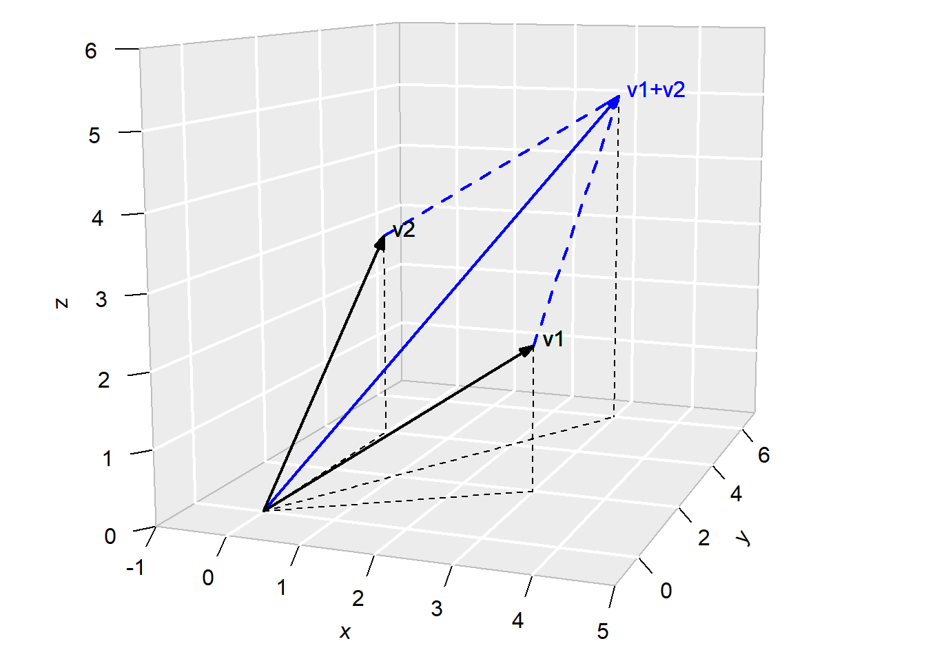
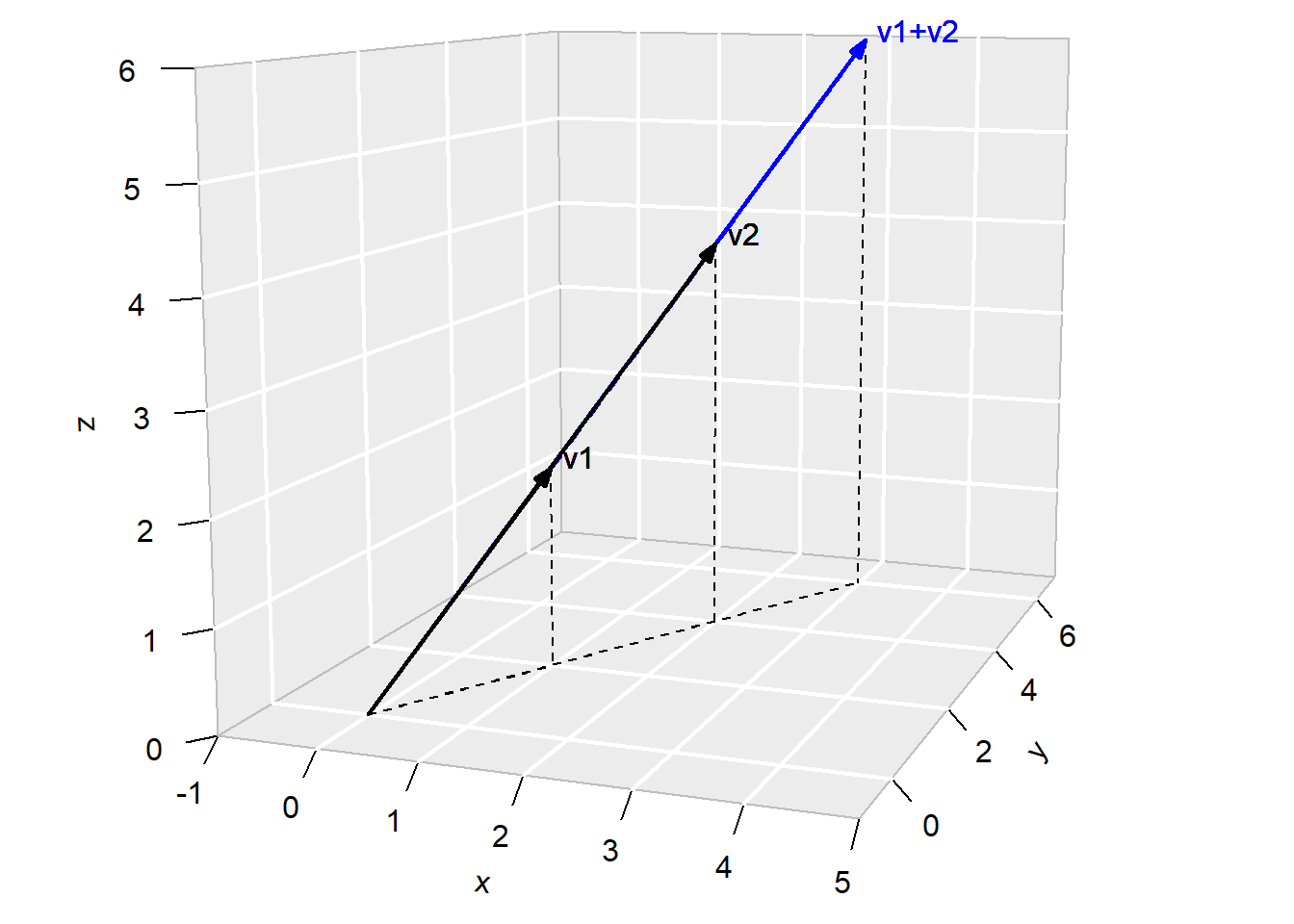
\] The result is a third vector that is a diagonal of the parallelogram formed by \(c_1v_1\) and \(c_2v_2\). This is illustrated in Fig. 8.4, which shows two vectors \[
v_1 = \begin{bmatrix} 3 \\ 2 \\ 2 \end{bmatrix}\,,\,\,
v_2 = \begin{bmatrix} 0 \\ 4 \\ 3 \end{bmatrix}
\] and their sum.
Figure 8.4: Linear combination of two 3-d vectors.
The three vectors \(v_1\), \(v_2\) and \(v_1+v_2\) all lie on the same plane. In fact, if we consider the set of all linear combinations of \(v_1\) and \(v_2\)\[
c_1 v_1 + c_2 v_2
\] we will find the this set makes up the entire plane containing \(v_1\) and \(v_2\). We say that these two 3-d vectors span the (2-dimensional) plane just described.
If the two vectors \(v_1\) and \(v_2\) are such that \(v_2 = cv_1\), then the two vectors lie on a line, and their linear combinations would also lie on the same line: \[
\text{if}\;\;
v_1 = \begin{bmatrix} 1 \\ 2 \\ 2 \end{bmatrix},
v_2 = \begin{bmatrix} 2 \\ 4 \\ 4 \end{bmatrix},
\;\;\text{ then }\;\;
v_3 = c_1v_1 + c_2v_2 = (c_1+2c_1)\begin{bmatrix} 1 \\ 2 \\ 2 \end{bmatrix}.
\]
Figure 8.5: A one-dimensional line spanned by two vectors.
Fig. 8.5 shows the vectors \(v_{1}\), \(v_{2}\) and \(v_{1}+v_{2}\). The set of linear combinations of \(v_1\) and \(v_2\) spans a (one-dimensional) line, not a two-dimensional plane. The same is true if one of the vectors is the zero vector, and the other is non-zero. If both are zero vectors, then the linear combinations are always just the zero vector. We say that the \((3 \times 2)\) matrix \[
A =
\begin{bmatrix}
v_{11} & v_{12} \\ v_{21} & v_{22} \\ v_{31} & v_{32}
\end{bmatrix}
\] has column rank two if its columns span a plane. It has column rank one if its columns span a line, and it has column rank zero if both columns are zero vectors.
Linear combinations of two 3-dimensional vectors, of course, cannot span the entire space – the highest dimensional space it can span is a two-dimensional plane. To span the entire three dimensional space, we need three vectors, and these three vectors cannot all lie on a plane or a line, and none of the vectors can be the zero vector. We say that the \((3 \times 3)\) matrix \[
A =
\begin{bmatrix}
v_{11} & v_{12} &v_{13} \\
v_{21} & v_{22} & v_{23} \\
v_{31} & v_{32} & v_{33}
\end{bmatrix}
=
\begin{bmatrix}
v_1 & v_2 & v_3
\end{bmatrix}
\] has column rank three, or full column rank, if the three column vectors that make up the matrix span the entire three dimensional space.
If the three column vectors span only 2-dimensions or less, then the three vectors all lie on the same plane or on a line, or are all zero. A compact way to describe these situations as a whole is that there is some \((c_1,c_2,c_3) \neq (0,0,0)\) such that \[
c_1 v_1 + c_2 v_2 + c_3 v_3 = 0\,,
\] that is, there is some \(c \neq 0\) such that \(Ac=0\). If the vectors are non-zero and all lie on a plane or a line, then one can be written as a linear combination of the other, thus \[
v_i = c_j v_j + c_k v_k\;\;\text{where}\;\;i,j,k = 1,2,3, \;\;\text{with}\;\;i \neq j \neq k \neq i\,,
\tag{8.3}\] or \(v_i - c_j v_j - c_k v_k = 0\). If one is a zero vector, say, \(v_1\), then we can write \(v_1 = 0v_2 + 0v_3\), or \(v_i - 0 v_j - 0 v_k = 0\). In all of these cases we have found \(c\neq 0\) such that \(Ac=0\). In these cases we say that the vectors \(v_1\), \(v_2\) and \(v_3\) are linearly dependent. On the other hand, if the three vectors span the entire 3-d space, then we cannot write one as a linear combination of the others. An expression like (8.3) will hold only when \(c=0\), i.e., \(Ac \neq 0\) for all \(c \neq 0\). In this case we say that the vectors are linearly independent.
What if we have a \((3 \times n)\) matrix where \(n>3\)? These vectors that make up the matrix may span the entire 3-d space (the matrix has rank 3), a 2-d plane (the matrix has column rank 2), or a 1-d line (the matrix has column rank 1). If all of the vectors are zero vectors, the matrix has column rank zero. Three-dimensional vectors, of course, cannot span a space of dimension greater than three. The column rank of an \((3 \times n)\) matrix cannot exceed 3.
We lose the literal geometric viewpoint once we enter the realm of higher-dimensional vectors, but the geometric intuition carries over. For instance, the two vectors \[
v_1 = \begin{bmatrix} 1 \\ 2 \\ 2 \\3 \end{bmatrix},
v_2 = \begin{bmatrix} 2 \\ 4 \\ 4 \\ 6\end{bmatrix},
\] span only a 1-d “line” (in 4-d space). Since \(v_2 = 2v_1\), every linear combination is also just a multiple of \(v_1\): \[
c_1 v_1 + c_2v_2 = c_1 v_1 + 2c_2v_1 = (c_1 + 2c_2)v_1\,.
\] The matrix \[
A = \begin{bmatrix} 1 & 2 \\ 2 & 4 \\ 2 & 4 \\3 & 6 \end{bmatrix}
\] therefore only has column rank one. On the other hand, the columns of the matrix \[
B = \begin{bmatrix} 1 & 2 \\ 2 & 4 \\ 2 & 4 \\3 & 5 \end{bmatrix}
\] span a 2-d “plane” in 4-d space; its column rank is two. A \((4 \times 3)\) matrix can have column ranks 0, 1, 2, or 3. The following matrices have column ranks 2 and 3 respectively: \[
C = \begin{bmatrix} 1 & 3 & 6 \\ 2 & 2 & 8 \\ 3 & 1 & 10\\4 & 1 & 13 \end{bmatrix} \,,\;\;
D = \begin{bmatrix} 1 & 0 & 0 \\ 0 & 1 & 0 \\ 0 & 0 & 1\\3 & 5 & 6 \end{bmatrix} .
\] A \((4 \times 4)\) matrix can have column rank 0 to 4. A \((4 \times n)\) matrix, where \(n>4\) can have column ranks 0 up to 4. In general, the rank of an \((m \times n)\) matrix cannot exceed the minimum of \(m\) and \(n\): \[
\mathrm{col.rank}(A) \leq \min(m,n).
\] If \(\mathrm{col.rank}(A) = n\), then \(Ac \neq 0\) for all \(c \neq 0\). If \(\mathrm{col.rank}(A) < n\), then there is a \(c \neq 0\) such that \(Ac = 0\).
8.1.2 The Rank of a Matrix
We could have done all this by treating a matrix as a collection of row vectors. For example, \[
A =
\begin{bmatrix}
v_{11} & v_{12} \\ v_{21} & v_{22} \\ v_{31} & v_{32}
\end{bmatrix}
=
\begin{bmatrix}
\begin{bmatrix} v_{11} & v_{12} \end{bmatrix}
\\ \begin{bmatrix} v_{21} & v_{22} \end{bmatrix}
\\ \begin{bmatrix} v_{31} & v_{32} \end{bmatrix}
\end{bmatrix}
=
\begin{bmatrix}
\mathrm{v}_1^\mathrm{T} \\
\mathrm{v}_2^\mathrm{T} \\
\mathrm{v}_3^\mathrm{T}
\end{bmatrix}
\] Linear combinations of the component row vectors can be written \(c^\mathrm{T}A\). We can talk about the linear dependence or linear independence of the row vectors, and the dimension of the space spanned by the vectors. All this leads to the concept of row rank. In general, the rank of an \((m \times n)\) matrix cannot exceed the minimum of \(m\) and \(n\): \[
\mathrm{row.rank}(A) \leq \min(m,n).
\] If \(\mathrm{row.rank}(A) = m\), then \(c^\mathrm{T}A \neq 0\) for all \(c \neq 0\).
Finally, we note that the row and column ranks of a matrix are always equal. Suppose the column rank of a matrix \(A\) is \(r \leq \min(m,n)\). This means you can find \(r\) linearly independent columns in \(A\). Collect these columns into the \((m \times r)\) matrix \(C\). Since every column in \(A\) can be written as a linear combination of the columns of \(C\), we can write \(A=CR\) for some \((r \times n)\) matrix \(R\). This in turn says that every row in \(A\) can be written as a linear combination of the rows of \(R\). Since there are only \(r\) rows in \(R\), it must be that the row rank of \(A\) is less than or equal to \(r\). That is, \[
\mathrm{row.rank}(A) \leq \mathrm{col.rank}(A).
\tag{8.4}\] Applying the same argument to \(A^\mathrm{T}\), we get \[
\mathrm{row.rank}(A^\mathrm{T}) \leq \mathrm{col.rank}(A^\mathrm{T}).
\] Since the row rank of a transpose is the column rank of the original matrix, we have \[
\mathrm{col.rank}(A) \leq \mathrm{row.rank}(A).
\tag{8.5}\] Inequalities (8.4) and (8.5) imply \[
\mathrm{row.rank}(A) = \mathrm{col.rank}(A).
\] We can therefore speak unambiguously of the rank of a matrix \(A\).
We state without proof a few results regarding the rank of a matrix:
For any matrices \(A\) and \(B\) for which \(AB\) exists, we have \[
\mathrm{rank}(AB) \leq \min(\mathrm{rank}(A), \mathrm{rank}(B)).
\]
A square matrix \(A\) has an inverse if and only if it is full rank.
If \(A\) is a full rank \((m \times m)\) matrix, and \(B\) is an \((m \times n)\) matrix of rank \(r\), then \(\mathrm{rank}(AB)=r\).
For any \((n \times k)\) matrix \(A\), we have \[
\mathrm{rank}(A^\mathrm{T}A) = \mathrm{rank}(A).
\] This means that \(A^\mathrm{T}A\) will have an inverse if and only if \(A\) has full column rank.
8.1.3 Finding the Rank of a Matrix in R
To find the rank of a matrix in R, we can feed the matrix into the qr() function, which returns a number of things, including the matrix’s rank.
Example 8.1 Use R to find the rank of the matrix \[
E = \begin{bmatrix} 2 & 2 & 4 \\ 2 & 1 & 3 \\ 2 & 5 & 7 \end{bmatrix}.
\]
E <-matrix(c(2,2,2,2,1,5,4,3,7),3,3)E_qr <-qr(E)E_qr$rank
[1] 2
8.1.4 Exercises
Exercise 8.1 The following matrices have rank one: \[
A = \begin{bmatrix} a_{11} & \alpha a_{11} \\ a_{21} & \alpha a_{21} \end{bmatrix},
B = \begin{bmatrix} a_{11} & 0 \\ a_{21} & 0 \end{bmatrix},
C = \begin{bmatrix} 0 & a_{12} \\ 0 & a_{22} \end{bmatrix}.
\] In each case find a non-zero \((2 \times 1)\) vector \(c\) such that \(Ac=0\). Show that in each case the determinant of the matrix is zero (so that the inverse does not exist).
Exercise 8.2 Suppose the matrix \[
A = \begin{bmatrix} a_{11} & a_{12} \\ a_{21} & a_{22} \end{bmatrix}
\] is such that \(a_{11}a_{22}-a_{12}a_{21} \neq 0\). Show that it cannot be that
one or more of the rows or columns have all zero entries;
one of the rows / columns is a multiple of the other row / column.
Show that the only \(c\) such that \(Ac=0\) is \(c=0\).
Exercise 8.3 What is the rank of the following matrices? (Try without using R.)
Exercise 8.4 Let \(\{X_i\}_{i=1}^N\) be a set of numbers, and consider the matrix \[
A = \begin{bmatrix}
N & \sum_{i=1}^N X_i \\
\sum_{i=1}^N X_i & \sum_{i=1}^N X_i^2
\end{bmatrix}
\] Show that \(A\) is rank one if and only if \(X_i\) is constant over all \(i\), i.e., \(X_i = b\), \(i=1,2,...,N\).
Exercise 8.5 Suppose \(A\) is a \((n \times n)\) diagonal matrix with \(r\) non-zero terms and \(n-r\) zero terms in its diagonal. What is its rank?
8.2 Diagonalization of Symmetric Matrices
A square matrix \(A\) is diagonalizable if it can be written in the form \[
A = C \Lambda C^{-1} \;\;\text{where}\;\;\Lambda\;\;\text{is diagonal}\,.
\tag{8.6}\] For such matrices, we have \(C^{-1}AC = \Lambda\). We will not prove this statement, except to note that the diagonal elements of \(\Lambda\) are the eigenvalues of \(A\), and the columns of \(C\) are the corresponding eigenvectors of \(A\). The decomposition (8.6) is called the eigen-decomposition of the matrix \(A\).
If the matrix \(A\) is symmetric, then we have in addition that \(C^{-1} = C^{\mathrm{T}}\), i.e., a symmetric matrix \(A\) can be written as \[
A = C \Lambda C^\mathrm{T} \;\; \text{ where } \;\;C^\mathrm{T}C = CC^\mathrm{T}=I\;\;\text{and}\;\; \Lambda\;\;\text{is diagonal}\,.
\tag{8.7}\] We say that \(A\) is orthogonally diagonalizable. Symmetric matrices are the only such matrices, i.e., a square matrix is orthogonally diagonalizable if and only if it is symmetric. Furthermore, the values of \(C\) and \(\Lambda\) will be real; if \(A\) is not symmetric, the eigenvalues and eigenvectors may be complex-valued.
If (8.7) holds for the \((n \times n)\) symmetric matrix \(A\), we can write \[
A = C\Lambda C^{\mathrm{T}} =
\begin{bmatrix} c_1 & c_2 & \dots & c_n \end{bmatrix}
\begin{bmatrix} \lambda_1 & 0 & \dots & 0 \\
0 & \lambda_2 & \dots & 0 \\
\vdots & \vdots & \ddots & \vdots \\
0 & 0 & \dots & \lambda_n
\end{bmatrix}
\begin{bmatrix} c_1^{\mathrm{T}} \\ c_2^{\mathrm{T}} \\ \dots \\ c_n^{\mathrm{T}} \end{bmatrix}
= \sum_{i=1}^{n} \lambda_i c_{i}c_{i}^{\mathrm{T}}\,.
\] where \(c_1, c_2, \dots, c_n\) are the \((n \times 1)\) columns of \(C\), and \(\lambda_1, \lambda_2,\dots, \lambda_n\) are the diagonal elements of \(\Lambda\).
A matrix \(C\) such that \(C^{\mathrm{T}}C = I\) is called orthogonal (sometimes orthonormal) because \[
C^{\mathrm{T}}C
=
\begin{bmatrix} c_1^{\mathrm{T}} \\ c_2^{\mathrm{T}} \\ \dots \\ c_n^{\mathrm{T}} \end{bmatrix}
\begin{bmatrix} c_1 & c_2 & \dots & c_n \end{bmatrix}
=
\begin{bmatrix}
c_1^\mathrm{T}c_1 & c_1^\mathrm{T}c_2 & \dots & c_1^\mathrm{T}c_n \\
c_2^\mathrm{T}c_1 & c_2^\mathrm{T}c_2 & \dots & c_2^\mathrm{T}c_n \\
\vdots & \vdots & \ddots & \vdots \\
c_n^\mathrm{T}c_1 & c_n^\mathrm{T}c_2 & \dots & c_n^\mathrm{T}c_n \\
\end{bmatrix}
=
\begin{bmatrix}
1 & 0 & \dots & 0 \\
0 & 1 & \dots & 0 \\
\vdots & \vdots & \ddots & \vdots \\
0 & 0 & \dots & 1 \\
\end{bmatrix}\,.
\] In other words, the columns of \(C\) are unit length vectors, and orthogonal to each other.
Example 8.2 For the matrix \[
A = \begin{bmatrix} 1 & 0 & 1 \\ 0 & 2 & 4 \\ 1 & 4 & 1 \end{bmatrix}.
\] the matrices \(C\) and \(\Lambda\) are \[
C \approx
\begin{bmatrix}
-0.1437 & 0.9688 & 0.2021 \\
-0.7331 & -0.2414 & 0.6359 \\
-0.6648 & 0.0568 & -0.7449
\end{bmatrix},
\Lambda \approx
\begin{bmatrix}
5.6272 & 0 & 0 \\
0 & 1.0586 & 0 \\
0 & 0 & -2.6858
\end{bmatrix}
\] which we can find from the following code
A=matrix(c(1,0,1,0,2,4,1,4,1), nrow=3)E=eigen(A)C <- E$vectors # E$vectors is CLambda <-diag(E$values) # E$values is diag values of \Lambdacat("C = \n"); round(C,4)
cat("\nVerifying A = C Lambda t(C): \n"); round(C %*% Lambda %*%t(C), 4)
Verifying A = C Lambda t(C):
     [,1] [,2] [,3]
[1,]    1    0    1
[2,]    0    2    4
[3,]    1    4    1
cat("\nVerifying C %*% t(C) = I: \n"); round(C %*%t(C), 4)
Verifying C %*% t(C) = I:
     [,1] [,2] [,3]
[1,]    1    0    0
[2,]    0    1    0
[3,]    0    0    1
The columns of \(C\) are the eigenvectors, and the diagonal elements of \(\Lambda\) are the eigenvalues of \(A\).
The diagonalization result (8.6) has many applications:
Suppose you want to find the 100th power of \(A\). Since \(A = C \Lambda C^{-1}\), we have \[
A = C \Lambda C^{-1}C \Lambda C^{-1} \dots C \Lambda C^{-1} = C\Lambda^{100}C^{-1}.
\] This is a much more efficient (and accurate) way of computing large powers of matrices than brute force multiplication.
Since \(AC = C\Lambda\) and \(C\) is full rank, \(A\) and \(\Lambda\) have the same rank. Since \(\Lambda\) is diagonal, its rank is just the number of non-zero elements in its diagonal. Therefore the rank of \(A\) is the number of non-zero elements in the diagonal of \(\Lambda\).
The determinant of the product of square matrices is the product of their determinants. Since \(AC = C\Lambda\), we have \(|A||C| = |C||\Lambda|\), from which it follows that \(|A| = |\Lambda|\). Furthermore, the determinant of a diagonal matrix is just the product of the diagonal elements.
Recall that a \((n \times n)\) matrix \(A\) is positive definite if \(c^\mathrm{T}Ac > 0\) for all vectors \(c \neq 0\). If \(A\) is symmetric, so that (8.7) holds, then we have \[
c^\mathrm{T}Ac = c^\mathrm{T}CC^{\mathrm{T}}ACC^{\mathrm{T}}c=b^\mathrm{T}\Lambda b = \sum_{i=1}^n b_i^2 \lambda_i
\] where \(b=C^{\mathrm{T}}c\). Since \(C^{\mathrm{T}}\) is invertible, it has full rank, which means that \(b=C^{\mathrm{T}}c \neq 0\) for all \(c \neq 0\), and it follows that \(\sum_{i=1}^n b_i^2 \lambda_i>0\) if \(\lambda_i>0\) for all \(i\). If \(\lambda_i \leq 0\) for one or more \(i\), then we can find \(b \neq 0\) (and therefore a \(c \neq 0\)) such that \(\sum_{i=1}^n b_i^2 \lambda_i \leq 0\). In other words, \(A\) is positive definite if and only if the diagonal elements of \(\Lambda\) are positive.
Since the diagonal elements of \(\Lambda\) are positive if \(A\) is symmetric and positive definite, we can write \(\Lambda = \Lambda^{1/2}\Lambda^{1/2}\). The matrix \(\Lambda^{1/2}\) is the diagonal matrix whose diagonal elements are the square root of the diagonal elements of \(\Lambda\). Then we have \[
A = C \Lambda^{1/2} \Lambda^{1/2} C^{\mathrm{T}} \;\; \text{ or } \;\; \Lambda^{-1/2}C^\mathrm{T} A C \Lambda^{-1/2} = I.
\] If we let \(P = \Lambda^{-1/2}C^\mathrm{-1}\), then we can write \[
PAP^\mathrm{T} = I \;\; \text{ or } \;\; A = P^{-1}(P^\mathrm{T})^{-1} = P^{-1}(P^{-1})^\mathrm{T} \;\;\text{ or } A^{-1} = P^\mathrm{T}P\,.
\]
What are these eigenvalues and eigenvectors? Think of a square matrix \(A\) as something that transforms one vector into another, i.e., \(Ax_1 = x_2\). In general, the new vector \(x_2\) will have a different length and a different direction from \(x_1\), i.e., in general there will be scaling and rotation. However, for any given matrix \(A\), there will be certain vectors \(x\) such that \[
Ax = \lambda x
\tag{8.8}\] where \(\lambda\) is a scalar. Recall that a scalar multiple of a vector only scales the vector, and reverses its direction if the scalar is negative. What (8.8) says is that \(Ax\) only stretches or shrinks the vector \(x\), without rotation (apart from possibly reversing the direction). Vectors \(x\) for which (8.8) holds are called the eigenvectors of \(A\), and the corresponding \(\lambda\)s are the eigenvalues.
8.2.1 Exercises
Exercise 8.6 A \((n \times n)\) matrix \(A\) is positive semidefinite if \(c^\mathrm{T}Ac \geq 0\) for all vectors \(c \neq 0\). Explain why a symmetric matrix \(A\) is positive semidefinite if and only if \(\lambda_i\) is non-negative for all \(i\).
Exercise 8.7 A square matrix \(A\) is said to be idempotent if \(AA=A\). For example, suppose \(X\) is \((N \times K)\) such that the \((K \times K)\) matrix \(X^\mathrm{T}X\) has an inverse (i.e., \(X\) has full column rank). Then the matrix \(A=X(X^\mathrm{T}X)^{-1}X^\mathrm{T}\) is idempotent, since \[
AA = X(X^\mathrm{T}X)^{-1}X^\mathrm{T}X(X^\mathrm{T}X)^{-1}X^\mathrm{T}=X(X^\mathrm{T}X)^{-1}X^\mathrm{T} = A.
\] Now suppose that \(A\) is idempotent and symmetric, and consider the diagonalization of this matrix: \[
C^\mathrm{T}AC = \Lambda.
\]
Explain why the diagonal elements of \(\Lambda\) can only take values \(1\) and \(0\). (Hint: We have \(AC=C\Lambda\), therefore \(AAC = AC\Lambda = C\Lambda^2\). Since \(AA=A\), we have \(AC=C\Lambda^2\). Since \(C\Lambda = C\Lambda^2\) and \(C\) is full rank, therefore \(\Lambda = \Lambda^2\).)
Show that the rank of a symmetric idempotent matrix \(A\) is equal to its trace. (Hint: \(\mathrm{tr}(A) = \mathrm{tr}(C\Lambda C^\mathrm{T}) = \mathrm{tr}(C^\mathrm{T}C\Lambda) = \mathrm{tr}(\Lambda)\).)
8.3 Differentiation of Matrix Forms
8.3.1 Definitions
This topic is easier that it sounds. What we mean by differentiation of matrix forms is merely a set of formulas that organize partial derivatives of functions written with matrices. For instance, for the function \(y = f(x_1,x_2, \dots x_n)\), which we write as \(f(x)\) where \(x^\mathrm{T}=\begin{bmatrix} x_1 & x_2 & \dots & x_n\end{bmatrix}\), we define the derivative of \(y\) with respect to the vector \(x\) to be \[
\frac{dy}{dx}
= \begin{bmatrix} \dfrac{\partial y}{\partial x_1} \\
\dfrac{\partial y}{\partial x_2} \\
\vdots \\
\dfrac{\partial y}{\partial x_n}
\end{bmatrix}
\hspace{0.5cm} \text{ and } \hspace{0.5cm}
\frac{dy}{dx^\mathrm{T}}
= \begin{bmatrix} \dfrac{\partial y}{\partial x_1} &
\dfrac{\partial y}{\partial x_2} &
\dots & \dfrac{\partial y}{\partial x_n}
\end{bmatrix}.
\] If \(y=f(x_1,x_2,x_3,x_4)\) and if \[
X = \begin{bmatrix} x_1 & x_2 \\ x_3 & x_4 \end{bmatrix},
\] then we define \[
\frac{dy}{dX}
= \begin{bmatrix} \dfrac{\partial y}{\partial x_1} & \dfrac{\partial y}{\partial x_2}\\
\dfrac{\partial y}{\partial x_3} & \dfrac{\partial y}{\partial x_4}
\end{bmatrix}.
\] Likewise if \(X\) is an \((m \times n)\) matrix.
Example 8.3 Let \[
X = \begin{bmatrix} x_1 & x_2 \\ x_3 & x_4 \end{bmatrix}
\] and \(y = |X| = x_1x_4-x_2x_3\). Then \[
\frac{dy}{dX}
= \begin{bmatrix} \dfrac{\partial y}{\partial x_1} & \dfrac{\partial y}{\partial x_2}\\
\dfrac{\partial y}{\partial x_3} & \dfrac{\partial y}{\partial x_4}
\end{bmatrix}
= \begin{bmatrix}
x_4 & -x_3 \\ -x_2 & x_1
\end{bmatrix}\,.
\] Since \[
X^{-1} = \frac{1}{|X|}\begin{bmatrix} x_4 & -x_2 \\ -x_3 & x_1 \end{bmatrix}
\] we have the formula \[
\frac{d}{dX}|X| = |X|(X^{-1})^\mathrm{T}.
\] This result holds for general non-singular square matrices (proof omitted).
8.3.2 Basic Differentiation Formulas
If \(y = f(x) = Ax\) where \(A = (a_{ij})_{mn}\) is a \((m \times n)\) matrix of constants and \(x = \begin{bmatrix} x_1 & x_2 & \dots & x_n \end{bmatrix}^\mathrm{T}\) is an \((n \times 1)\) vector of variables, then \[
\dfrac{dy}{dx^\mathrm{T}} = A\,.
\tag{8.9}\]Proof: The \(ith\) element of \(Ax\) is \(\sum_{k=1}^n a_{ik}x_k\). Therefore the \((i,j)th\) element of \(\dfrac{dy}{dx^\mathrm{T}}\) is \[
\frac{\partial}{\partial x_j}\sum_{k=1}^n a_{ik}x_k = a_{ij}
\] which says that \(\dfrac{dy}{dx^\mathrm{T}}=A\). Result (8.9) is the matrix analogue of the univariate differentiation rule \(\frac{d}{dx}ax = a\).
If \(y = f(x) = x^\mathrm{T}Ax\) where \(A = (a_{jk})_{nn}\) is a \((n \times n)\) matrix of constants, then \[
\dfrac{dy}{dx} = \dfrac{d}{dx}x^\mathrm{T}Ax = (A+A^\mathrm{T})x.
\tag{8.10}\]Proof:\(y = x^\mathrm{T}Ax = \sum_{j=1}^n \sum_{k=1}^n a_{jk}x_jx_k\). The derivative \(\frac{dy}{dx}\) is the \((n \times 1)\) vector whose \(ith\) element is \[
\frac{d}{dx_i}\sum_{j=1}^n \sum_{k=1}^n a_{jk}x_jx_k
= \sum_{k=1}^n a_{ik}x_k + \sum_{j=1}^n a_{ji}x_j.
\] The first sum after the equality is the product of the \(ith\) row of \(A\) into \(x\). The second sum after the inequality is the product of the \(ith\) row of \(A^\mathrm{T}\) into \(x\). In other words, \(\dfrac{dy}{dx} = (A+A^\mathrm{T})x\).
It may be helpful to derive this formula by direct differentiation in a special case, say, where \(A\) is \((3 \times 3)\). You are asked to do this in an exercise. Note that if \(A\) is symmetric, then (8.10) becomes \[
\dfrac{dy}{dx} = \dfrac{d}{dx}x^\mathrm{T}Ax = (A+A^\mathrm{T})x = 2Ax.
\tag{8.11}\] The result then becomes directly comparable to the univariate differentiation rule \(\frac{d}{dx}ax^2 = 2ax\).
If \(y = f(x)\) is a scalar valued function of an \((n \times 1)\) vector of variables, then \[
\dfrac{d}{dx^\mathrm{T}}\left( \frac{dy}{dx}\right)
= \dfrac{d}{dx^\mathrm{T}}
\begin{bmatrix} \dfrac{dy}{dx_1} \\ \dfrac{dy}{dx_2} \\ \vdots \\ \dfrac{dy}{dx_n}
\end{bmatrix}
= \begin{bmatrix}
\dfrac{d^2y}{dx_1^2} & \dfrac{d^2y}{dx_1dx_2} & \dots & \dfrac{d^2y}{dx_1dx_n} \\
\dfrac{d^2y}{dx_2dx_1} & \dfrac{d^2y}{dx_2^2} & \dots & \dfrac{d^2y}{dx_2dx_n} \\
\vdots & \vdots & \ddots & \vdots \\
\dfrac{d^2y}{dx_ndx_1} & \dfrac{d^2y}{dx_ndx_2} & \dots & \dfrac{d^2y}{dx_n^2}
\end{bmatrix}.
\tag{8.12}\]
In other words, we get the Hessian matrix of \(y\). We write \(\dfrac{d}{dx^\mathrm{T}}\left( \dfrac{dy}{dx}\right)\) as \[
\dfrac{d}{dx^\mathrm{T}}\left( \frac{dy}{dx}\right) = \frac{d^2y}{dxdx^\mathrm{T}}.
\]
8.3.3 Exercises
Exercise 8.8 Show that if \(y = f(x) = x^\mathrm{T}A\) where \(A = (a_{ij})_{mn}\) is a \((m \times n)\) matrix of constants and \(x = \begin{bmatrix} x_1 & x_2 & \dots & x_m \end{bmatrix}^\mathrm{T}\) is an \((m \times 1)\) vector of variables, then \[
\dfrac{dy}{dx} = A\,.
\]
Exercise 8.9 If \(c\) is an \(n\)-dimensional vector of constants and \(x\) is an \(n\)-dimensional vector of variables, show that \[
\dfrac{d}{dx}c^\mathrm{T}x = c\,.
\]
Exercise 8.10 Let \(A=(a_{ij})_{33}\) be a \((3 \times 3)\) matrix of constants, and \(x\) be a \((3 \times 1)\) vector of variables. Multiply out \(x^\mathrm{T}Ax\) in full, and show by direct differentiation that \[
\dfrac{dy}{dx} = (A+A^\mathrm{T})x\,.
\]
Exercise 8.11 Use the fact that \(\frac{d}{dX}|X| = |X|(X^{-1})^\mathrm{T}\) for a general square matrix \(X\) to show that if \(|X|>0\), then \[
\frac{d}{dX}\ln|X| = (X^{-1})^\mathrm{T}\,.
\]
Exercise 8.12 Show that if \(A=(a_{ij})_{nn}\) is an \((n\times n)\) matrix of constants and \(x\) is an \(n\)-dimensional vector of variables, then \[
\frac{d^2 (x^\mathrm{T}Ax)}{dxdx^\mathrm{T}} = A + A^\mathrm{T}\,.
\]
Exercise 8.13 Show that for any \((n \times n)\) square matrix \(A\), we have \[
\frac{d\mathrm{tr}(A)}{dA} = I_n\,.
\]
8.4 Vectors and Matrices of Random Variables
Organizing large numbers of random variables using matrix algebra provides convenient formulas for manipulating their expectations, variances and covariances, and for expressing their joint pdf.
8.4.1 Expectations and Variance-Covariance Matrices
The expectation of a vector \(x\) of \(M\) random variables \[
x = \begin{bmatrix} X_1 & X_2 & \dots & X_M \end{bmatrix}^\mathrm{T}
\] is defined as the vector of their expectations, i.e., \[
E[x] = \begin{bmatrix} E[X_1] & E[X_2] & \dots & E[X_M] \end{bmatrix}^\mathrm{T}.
\]
Likewise, if \(X\) is a matrix of random variables \[
X = \begin{bmatrix}
X_{11} & X_{12} & \dots & X_{1N} \\
X_{21} & X_{22} & \dots & X_{2N} \\
\vdots & \vdots & \ddots & \vdots \\
X_{M1} & X_{M2} & \dots & X_{MN} \\
\end{bmatrix}
\] then \[
E[X] = \begin{bmatrix}
E[X_{11}] & E[X_{12}] & \dots & E[X_{1N}] \\
E[X_{21}] & E[X_{22}] & \dots & E[X_{2N}] \\
\vdots & \vdots & \ddots & \vdots \\
E[X_{M1}] & E[X_{M2}] & \dots & E[X_{MN}] \\
\end{bmatrix}.
\] With these definitions, we can define the variance-covariance matrix of a vector \(x\) of random variables. Let \[
\tilde{x}
= x - E[x]
= \begin{bmatrix}
X_1-E[X_1] \\ X_2-E[X_2] \\ \vdots \\ X_M-E[X_M]
\end{bmatrix}
= \begin{bmatrix}
\tilde{X}_1 \\ \tilde{X}_2 \\ \vdots \\ \tilde{X}_M
\end{bmatrix}
\] Then \[
\begin{aligned}
E[\tilde{x}\tilde{x}^\mathrm{T}]
= E[(x - E[x])(x - E[x])^\mathrm{T}]
&= E
\begin{bmatrix}
\tilde{X}_1^2 & \tilde{X}_1\tilde{X}_2 & \dots & \tilde{X}_1\tilde{X}_M \\
\tilde{X}_2\tilde{X}_1 & \tilde{X}_2^2 & \dots & \tilde{X}_2\tilde{X}_M \\
\vdots & \vdots & \ddots & \vdots \\
\tilde{X}_M\tilde{X}_1 & \tilde{X}_M\tilde{x}_2 & \dots & \tilde{X}_M\tilde{X}_M \\
\end{bmatrix} \\[2ex]
&= \begin{bmatrix}
E[\tilde{X}_1^2] & E[\tilde{X}_1\tilde{X}_2] & \dots & E[\tilde{X}_1\tilde{X}_M] \\
E[\tilde{X}_2\tilde{X}_1] & E[\tilde{X}_2^2] & \dots & E[\tilde{X}_2\tilde{X}_M] \\
\vdots & \vdots & \ddots & \vdots \\
E[\tilde{X}_M\tilde{X}_1] & E[\tilde{X}_M\tilde{X}_2] & \dots & E[\tilde{X}_M\tilde{X}_M] \\
\end{bmatrix} \\[2ex]
&= \begin{bmatrix}
var[X_1] & cov[X_1,X_2] & \dots & cov[X_1,X_M] \\
cov[X_1,X_2] & var[X_2] & \dots & cov[X_2,X_M] \\
\vdots & \vdots & \ddots & \vdots \\
cov[X_1,X_M] & cov[X_2,X_M] & \dots & var[X_M]
\end{bmatrix}\,.
\end{aligned}
\tag{8.13}\] In other words, \(E[(x - E[x])(x - E[x])^\mathrm{T}]\) is a symmetric matrix containing the variances of all of the variables in \(x\), and their covariances. We denote this matrix by \(var[X]\).
If \(X\) is a random variable (singular), then \(E[aX + b] = aE[X] + b\) and \(var[aX + b] = a^2var[X]\). The following are the matrix analogues: let \(x\) be an \((M \times 1)\) vector of random variables, and \(X\) be a \((K \times M)\) matrix of random variables. Let \(A=(a_{km})_{KM}\) be a \((K \times M)\) matrix of constants, and \(b\) be a \((K \times 1)\) vector of constants. Then
\(E[Ax + b] = AE[x] + b\)
Proof: \(Ax + b\) is a \((K \times 1)\) vector whose \(k\mathrm{th}\) element is \(\sum_{m=1}^M (a_{km}x_m + b_k)\), and the expectation of this term is \[
E\left[\sum_{m=1}^M (a_{km}x_m + b_k)\right]
= \sum_{m=1}^M a_{km}E[x_m] + b_k
\] which in turn is the \(k\mathrm{th}\) element of the vector \(AE[x] + b\).
\(var[Ax + b] = Avar[x]A^\mathrm{T}\)
Proof: Since \((Ax + b)-E[(Ax + b) = A(x-E[x]) = A\tilde{x}\), we have \[
var[Ax + b]
= E[(A\tilde{x})(A\tilde{x})^\mathrm{T}]
= E[A\tilde{x}\tilde{x}^\mathrm{T}A^\mathrm{T}]
= AE[\tilde{x}\tilde{x}^\mathrm{T}]A^\mathrm{T}
= Avar[x]A^\mathrm{T}\,.
\] If \(X\) is a random variable (singular), we have \(var[X] = E[X^2] - E[X]^2\). The matrix analogue of this result is \[
var[x] = E[xx^\mathrm{T}] - E[x]E[x]^\mathrm{T}
\tag{8.14}\] (see exercises).
Given a vector of random variables \(x\), the linear combination \(c^\mathrm{T}x\) has variance-covariance matrix \(c^\mathrm{T}var[x]c\). Since variances cannot be negative, we have \(c^\mathrm{T}var[x]c \geq 0\) for all \(c\). This means that \(var[x]\) is a positive semidefinite matrix. If there is a linear combination with zero variance, then at least one or more of the variables is actually a constant, or at least one or more of the variables is a linear combination of the others. Otherwise we have \(c^\mathrm{T}var[x]c > 0\) for all \(c \neq 0\), i.e., \(var[x]\) is positive definite.
Since \(var[x]\) is symmetric and positive definite, we can find a \(C\) such that \(C^\mathrm{T}var[x]C = \Lambda\) where \(\Lambda\) is diagonal. But \(C^\mathrm{T}var[x]C\) is the variance of \(C^\mathrm{T}x\). In other words, \(C^\mathrm{T}x\) is a vector of uncorrelated random variables, obtained from the (possibly) correlated random variables in \(x\). Furthermore, we have \(var[Px] = I\) where \(P = \Lambda^{-1/2}C^{\mathrm{T}}\).
8.4.2 The Multivariate Normal Distribution
We presented the pdf of a bivariate normal distribution in an earlier chapter. We present here the pdf of a general multivariate normal distribution and some associated results. A \((K \times 1)\) vector of random variables \(x\) is said to have a multivariate normal distribution with mean \(\mu\) and variance-covariance matrix \(\Sigma\), denoted \(\mathrm{Normal}_K(\mu,\Sigma)\), if its pdf has the form \[
f(x) = (2\pi)^{-K/2}|\Sigma|^{-1/2}\exp\left\{-\frac{1}{2}(x-\mu)^\mathrm{T}\Sigma^{-1}(x-\mu)\right\}
\] We list a few results below, omitting proofs:
If \(\Sigma\) is diagonal, then the variables are independent.
If \(x \sim \mathrm{Normal}_K(\mu, \Sigma)\), then \(Ax + b \sim \mathrm{Normal}_K(A\mu+b, A\Sigma A^\mathrm{T})\).
If we partition \(x\) as \[
\begin{bmatrix} x_1 \\ x_2 \end{bmatrix}
\sim
\mathrm{Normal}_K\left(
\begin{bmatrix}
\mu_1 \\ \mu_2
\end{bmatrix},
\begin{bmatrix}
\Sigma_{11} & \Sigma_{12} \\
\Sigma_{21} & \Sigma_{22}
\end{bmatrix}
\right)
\] where \(x_1\) is \((K_1 \times 1)\) and \(x_2\) is \((K_2 \times 1)\), with \(K_1 + K_2 = K\), then the marginal distribution of \(x_1\) is \(\mathrm{Normal}_{K_1}(\mu_1, \Sigma_{11})\), and the conditional distribution of \(x_2\) given \(x_1\) is \[
x_2 | x_1 \sim \mathrm{Normal}_{K_2}(\mu_{2|1}, \Sigma_{22|1})
\] where \[
\mu_{2|1} = \mu_2 + \Sigma_{21}\Sigma_{11}^{-1}(x_1-\mu_1)
\hspace{0.5cm}\text{and}\hspace{0.5cm}
\Sigma_{22|1} = \Sigma_{22} - \Sigma_{21}\Sigma_{11}^{-1}\Sigma_{12}.
\]
If \(x \sim \mathrm{Normal}_K(0,I)\) and \(A\) is symmetric and idempotent with rank \(J\), then the scalar \(x^\mathrm{T} A x\) is distributed \(\chi_{(J)}^2\).
If \(x \sim \mathrm{Normal}_K(\mu,\Sigma)\), then \[
(x-\mu)^\mathrm{T} \Sigma^{-1} (x-\mu) \sim \chi_{(K)}^2.
\]
8.4.3 Exercises
Exercise 8.14 Show that \(var[x] = E[xx^\mathrm{T}] - E[x]E[x]^\mathrm{T}\).
Exercise 8.15 Show that \(E[\mathrm{trace}[X]] = \mathrm{trace}[E[X]]\).
8.5 An Application of the Eigendecomposition of a Symmetric Matrix
Suppose \(X\) is a data matrix containing \(N\) observations of \(K\) variables \[
\begin{bmatrix}
X_{1,1} & X_{2,1} & \dots & X_{K,1} \\
X_{1,2} & X_{2,2} & \dots & X_{K,2} \\
\vdots & \vdots &\ddots & \vdots \\
X_{1,N} & X_{2,N} & \dots & X_{K,N}
\end{bmatrix}
=
\begin{bmatrix}
\mathrm{x}_{1} & \mathrm{x}_{2} & \dots \mathrm{x}_{K}
\end{bmatrix}
\;\; \text{where} \;\;
\mathrm{x}_k =
\begin{bmatrix}
X_{k,1} \\ X_{k,2} \\ \vdots \\ X_{k,N}
\end{bmatrix} \,.
\] Suppose that these variables have had their sample means removed, i.e., that \(X_{k,i}\) is actually \(X_{k,i} - \overline{X_{k}}\) where \(\overline{X_{k}} = (1/N)\sum_{i=1}^{N}X_{k,i}\). Furthermore, we assume that the variables have been standardized so that their individual sample variables are equal to 1.
Recall also that if you post-multiply \(X\) by a \((K \times 1)\) vector \(c\), you get a linear combination of the vectors of \(X\): \[
Xc
=
\begin{bmatrix}
\mathrm{x}_{1} & \mathrm{x}_{2} & \dots \mathrm{x}_{K}
\end{bmatrix}
\begin{bmatrix}
c_{1} \\ c_{2} \\ \vdots \\ c_{K}
\end{bmatrix}
=
\sum_{k=1}^{K} c_{k} \mathrm{x}_{k}\,.
\] You can think of this as a sample of observations of a new random variable \(Z = c_1X_1 + c_2X_2 + \dots c_{K}X_{K}\).
If you have a collection of \(J\) number of such \(c\) vectors, say \[
C = \begin{bmatrix} c_{1} & c_{2} & \dots & c_{J} \end{bmatrix}
\] where each of the \(c_1\), \(c_2\), …, \(c_J\) are now \((K\times 1)\) vectors, then \(XC\) contains the observations of \(J\) new variables, each of which is a linear combination of the \(X\) variables: \[
XC
=
X
\begin{bmatrix}
c_{1} & c_{2} & \dots & c_{J}
\end{bmatrix}
=
\begin{bmatrix}
Xc_{1} & Xc_{2} & \dots & Xc_{J}
\end{bmatrix}
\] Now consider the matrix \[
X^{\mathrm{T}}X
=
\begin{bmatrix}
\mathrm{x}_{1}^\mathrm{T} \\ \mathrm{x}_{2}^\mathrm{T} \\ \vdots \\ \mathrm{x}_{K}^\mathrm{T}
\end{bmatrix}
\begin{bmatrix}
\mathrm{x}_{1} & \mathrm{x}_{2} & \dots \mathrm{x}_{K}
\end{bmatrix}
=
\begin{bmatrix}
\mathrm{x}_{1}^\mathrm{T}\mathrm{x}_{1} & \mathrm{x}_{1}^\mathrm{T}\mathrm{x}_{2} & \dots & \mathrm{x}_{1}^\mathrm{T}\mathrm{x}_{K} \\
\mathrm{x}_{2}^\mathrm{T}\mathrm{x}_{1} & \mathrm{x}_{2}^\mathrm{T}\mathrm{x}_{2} & \dots & \mathrm{x}_{2}^\mathrm{T}\mathrm{x}_{K} \\
\vdots & \vdots & \ddots & \vdots \\
\mathrm{x}_{K}^\mathrm{T}\mathrm{x}_{1} & \mathrm{x}_{K}^\mathrm{T}\mathrm{x}_{2} & \dots & \mathrm{x}_{K}^\mathrm{T}\mathrm{x}_{K} \\
\end{bmatrix}\,.
\] Since the observations have been de-meaned, the terms \(\mathrm{x}_{k}^\mathrm{T}\mathrm{x}_{j} = \sum_{i=1}^{N} X_{k,i}X_{j,i}\) are just \(N\) times the sample covariance of \(X_{k}\) and \(X_{j}\), and \(\mathrm{x}_{k}^\mathrm{T}\mathrm{x}_{k} = \sum_{i=1}^{N} X_{k,i}^{2}\) is just \(N\) times the sample variance of \(X_{k}\). In other words, \((1/N) X^\mathrm{T} X\) is the sample variance-covariance matrix of the variables. To simplify notation, I will just drop the \((1/N)\) and refer to \(X^\mathrm{T} X\) as the sample variance-covariance matrix which summarizes the correlations between the variables in your data matrix \(X\).
Since \(X^\mathrm{T} X\) is symmetric, we can write \[
X^\mathrm{T} X = C \Lambda C^{\mathrm{T}} \;\;\text{where}\;\;CC^{\mathrm{T}} = I \,
\tag{8.15}\] and where \(\Lambda\) is a diagonal matrix containing the eigenvalues of \(X^\mathrm{T} X\), and the columns of \(C\) are the corresponding eigenvectors. Since \[
C\Lambda C^{\mathrm{T}} =
\begin{bmatrix} c_1 & c_2 & \dots & c_n \end{bmatrix}
\begin{bmatrix} \lambda_1 & 0 & \dots & 0 \\
0 & \lambda_2 & \dots & 0 \\
\vdots & \vdots & \ddots & \vdots \\
0 & 0 & \dots & \lambda_n
\end{bmatrix}
\begin{bmatrix} c_1^{\mathrm{T}} \\ c_2^{\mathrm{T}} \\ \dots \\ c_n^{\mathrm{T}} \end{bmatrix}
= \sum_{i=1}^{n} \lambda_i c_{i}c_{i}^{\mathrm{T}}\,
\] and since the terms of a summation can be added in any order, we can rearrange the columns of \(C\) in any order, as long as we also re-arrange the diagonals of \(\Lambda\) accordingly. We usually arrange it such that the eigenvalues are in descending order \(\lambda_1 \geq \lambda_2 \geq \dots \geq \lambda_K\).
The decomposition (8.15) can be re-written as \[
C^{\mathrm{T}}X^\mathrm{T} XC = \Lambda
\] or \[
(XC)^\mathrm{T} (XC) = \Lambda
\] This is just the sample covariance matrix of the variables whose observations appear in the columns of \(XC\). Each of the columns in \(XC\) are just linear combinations of the columns of \(X\). Since \(\Lambda\) is diagonal, this says that the \(K\) columns of \(XC\) are orthogonal. In other words, we have created \(K\)uncorrelated new variables, each of which is a linear combination of the (possibly correlated) \(X\) variables. Furthermore, writing the new variables as \[
XC = \begin{bmatrix} X c_{1} & X c_{2} & \dots & X c_{K} \end{bmatrix}
\] we see that \(\lambda_1\) is the sample variance of \(Xc_1\), \(\lambda_2\) is the sample variance of \(X c_{2}\), and so on.
The new variables in \(XC\) are called the principal components of \(X\). These are often used as a dimension reduction technique. Suppose \(X\) contains \(N\) observations of many many variables, so \(K\) is large. Quite often we find that only a few of the \(\lambda_i\)’s associated with \(X\) are large, and the rest very small. In other words, only a few of the principal components of \(X\) have substantial variation, the rest have very little variation. Sometimes just two or three of the principal components associated with the largest eigenvalues account for the bulk of variation in the data. If that is the case, then we have effectively reduced the number of variables from \(K\) to just two or three. The difficulty is that these principal components are often hard to interpret.
The code uses the package plot3D. The code for the figures are not shown, to avoid distracting from the main discussion.↩︎