library(tidyverse);
library(lmtest); library(sandwich); library(car)
library(ivreg); library(gmm)8 Instrumental Variables and GMM
We present the concept of instrumental variables, and an estimation method called Generalized Method of Moments (GMM). This extended framework enables consistent estimation of economic relationships in situations where there are endogeneity problems, i.e., where (for whatever reason) there are correlations between the noise term and one or more regressors. However, it requires the availability of good instrumental variables, which may not be so easy to find.
The R code in this chapter uses the packages
8.1 Using Instruments
Suppose you wish to estimate the simple linear regression \[ Y = \beta_0 + \beta_1 X + \epsilon\,. \tag{8.1}\] You are interested in estimating the effect that a change in \(X\) will have on \(Y\), but you strongly suspect that \(\epsilon\) is correlated with \(X\). This may be because of omitted factors (which for some reason you are unable to include, or because of measurement error, or perhaps there is simultaneity bias. This correlation between
Suppose, however, that there exists another variable \(Z\) such that \(\mathit{Cov}(X, Z) \neq 0\) and \(\mathit{Cov}(Z, \epsilon) = 0\). Such a variable is called an instrumental variable. It turns out that, if at least one such variable exists, we can use it to help us estimate \(\beta_1\), though there are trade-offs involved. We demonstrate this from two perspectives.
8.1.1 A Method of Moments Perspective
Suppose that in population we have \[ Y = \beta_0 + \beta_1 X + \epsilon\,. \tag{8.2}\] where \(\epsilon\) is zero mean but \(\epsilon\) is correlated with \(X\), but there there is another variable \(Z\) that is (i) correlated with \(X\) but (ii) uncorrelated with \(\epsilon\). We’ll make the slightly stronger assumption that \(E(\epsilon \mid Z) = 0\). This gives us the following “Population Moment Conditions”: \[ \begin{aligned} E(\epsilon) & = E(Y - \beta_0 - \beta_1 X) = 0 \\[1ex] E(\epsilon Z) & = E((Y - \beta_0 - \beta_1 X)Z) = 0 \end{aligned} \tag{8.3}\] Suppose that we have a iid sample \(\{Y_i, X_{i}, Z_i\}_{i=1}^n\) from the population. The method of moments approach is to choose as our estimators of \(\beta_0\) and \(\beta_1\) those values \(\widehat{\beta}_0^{mm}\) and \(\widehat{\beta}_1^{mm}\) such that the sample moments corresponding to (8.3), that is, \[ \begin{aligned} \frac{1}{n}\sum_{i=1}^{n} (Y_{i} - \hat{\beta}_0^{mm} - \hat{\beta}_1^{mm} X_{i}) = 0 \qquad&[A]\\[1ex] \frac{1}{n}\sum_{i=1}^{n} (Y_{i} - \hat{\beta}_0^{mm} - \hat{\beta}_1^{mm} X_{i})Z_{i} = 0 \qquad& [B] \end{aligned} \tag{8.4}\] Solving gives the method of moments (MM) estimator. From [A] we get \[ \overline{Y} = \hat{\beta}_0^{mm} - \hat{\beta}_1^{mm} \overline{X} \Rightarrow \hat{\beta}_0^{mm} = \overline{Y} - \hat{\beta}_1^{mm} \overline{X}\,. \] Substituting into [B] gives \[ \begin{gathered} \sum_{i=1}^{n} (Y_{i} - (\overline{Y} - \hat{\beta}_1^{mm} \overline{X}) - \hat{\beta}_1^{mm} X_{i})Z_{i} = 0 \\ \sum_{i=1}^{n} ((Y_{i} - \overline{Y}) - \hat{\beta}_1^{mm} (X_i - \overline{X}))Z_{i} = 0 \\ \sum_{i=1}^{n} (Y_{i} - \overline{Y})Z_i - \hat{\beta}_1^{mm} \sum_{i=1}^{n}(X_i - \overline{X})Z_{i} = 0\,. \end{gathered} \] Solving for \(\widehat\beta_0^{mm}\) and \(\widehat\beta_1^{mm}\) gives \[ \begin{aligned} \hat{\beta}_0^{mm} &= \overline{Y} - \hat{\beta}_1^{mm}\overline{X} \\[1ex] \hat{\beta}_1^{mm} &= \frac{\sum_{i=1}^n(Y_i - \overline{Y})Z_i} {\sum_{i=1}^n(X_i - \overline{X})Z_i} = \frac{\sum_{i=1}^n(Z_i - \overline{Z})(Y_i - \overline{Y})} {\sum_{i=1}^n(Z_i - \overline{Z})(X_i - \overline{X})} \end{aligned} \tag{8.5}\] These estimators are consistent. Focusing on \(\widehat{\beta}_1^{mm}\), we have \[ \begin{aligned} \hat{\beta}_1^{mm} &= \frac{\sum_{i=1}^n(Y_i - \overline{Y})Z_i} {\sum_{i=1}^n(X_i - \overline{X})Z_i} = \frac{\sum_{i=1}^n(Z_i - \overline{Z})Y_i} {\sum_{i=1}^n(Z_i - \overline{Z})X_i} \\[1ex] &= \frac{\sum_{i=1}^n(Z_i - \overline{Z})(\beta_0 + \beta_1X_i + \epsilon_i)} {\sum_{i=1}^n(Z_i - \overline{Z})X_i} \\[1ex] &= \beta_1 + \frac{\sum_{i=1}^n(Z_i - \overline{Z})\epsilon_i} {\sum_{i=1}^n(Z_i - \overline{Z})X_i} \;\overset{p}{\longrightarrow}\; \beta_1 + \frac{\mathit{Cov}(Z, \epsilon)}{{\mathit{Cov}(Z, X)}} = \beta_1 \end{aligned} \] since \(\mathit{Cov}(Z, \epsilon) = 0\) and (just as importantly) \(\mathit{Cov}(Z, X) \neq 0\)
Alternatively, you can show that \[ E(Y - \beta_0 - \beta_1 X) = 0 \text{ and } E((Y - \beta_0 - \beta_1 X)Z) = 0 \] implies \(\beta_1 = \mathit{Cov}(Z, Y) / \mathit{Cov}(Z,X)\) (see exercises). Then \[ \hat{\beta}_1^{mm} = \frac{\sum_{i=1}^n(Y_i - \overline{Y})(Z_i-\overline{Z})} {\sum_{i=1}^n(X_i - \overline{X})(Z_i-\overline{Z})} \;\overset{p}{\longrightarrow}\; \frac{\mathit{Cov}(Y, Z)}{\mathit{Cov}(X,Z)} = \beta_1 \]
8.1.2 A Two-Stage Least Squares Approach
Another way of using the instrumental variable is via “two-stage least squares” or 2SLS. We know that given \(X_i\) and \(Z_i\), we can decompose \(X_i\) into two perfectly uncorrelated parts by regressing \(X_i\) on \(Z_i\) by OLS, giving \[ X_i = \widehat{\delta}_0 + \widehat{\delta}_1Z_i + r_{i, x|z} = \hat{X}_i + r_{i, x|z}\,. \tag{8.6}\] Since \(\hat{X}_i\) is simply a linear function of \(Z_i\), and \(Z_i\) is uncorrelated with \(\epsilon_i\), so \(\hat{X}_i\) is uncorrelated with \(\epsilon_i\). In other words, all of the movements in \(X_i\) that are correlated with \(\epsilon_i\) are “concentrated” into \(r_{i, x|z}\). Alternatively, you can think of \(\hat{X}_i\) as that part of \(X_i\) that remains after filtering out the movements in \(X_i\) that are correlated with \(\epsilon_i\).
The idea is to use only the movements in \(X_i\) that are uncorrelated with \(\epsilon_i\) when determining the effect of \(X_i\) on \(Y_i\). In other words, we regress \(Y_i\) on \(\hat{X}_i\) instead of \(X_i\). This gives \[ \hat{\beta}_1^{2sls} = \frac{\sum_{i=1}^n(Y_i - \overline{Y})(\hat{X}_i-\overline{\hat{X}})}{\sum_{i=1}^n(\hat{X}_i - \overline{\hat{X}})^2} \;. \tag{8.7}\] This turns out to be equivalent to the MM estimator that we derived earlier. Since \(\hat{X}_i = \widehat{\delta}_0 + \widehat{\delta}_1Z_i\), we have \(\overline{\hat{X}} = \widehat{\delta}_0 + \widehat{\delta}_1 \overline{Z}\) and \[ \hat{X}_i - \overline{\hat{X}} = \widehat{\delta}_1 (Z_i - \overline{Z}) \] and \[ \sum_{i=1}^n(\hat{X}_i - \overline{\hat{X}})^2 = \widehat{\delta}_1^2 \sum_{i=1}(Z_i - \overline{Z})^2\,. \] Substituting into (8.7) gives \[ \hat{\beta}_1^{2sls} = \frac{\hat{\delta}_1\sum_{i=1}^T(Z_i-\overline{Z})(Y_i-\overline{Y})} {\hat{\delta}_1^2\sum_{i=1}^T(\hat{X}_t - \overline{\hat{X}})^2} = \frac{\sum_{i=1}^T(Z_i-\overline{Z})(Y_i-\overline{Y})} {\hat{\delta}_1\sum_{i=1}^T(\hat{X}_t - \overline{\hat{X}})^2} \,. \tag{8.8}\] Since \(\hat{\delta}_1\) is the OLS estimator for the coefficient on \(Z_i\) in a regression of \(X_i\) and \(Z_i\), we have \[ \hat{\delta}_1 = \frac{\sum_{i=1}^n(Z_i - \overline{Z})({X}_i-\overline{{X}})}{\sum_{i=1}^n({Z}_i - \overline{{Z}})^2}\,. \] Substituting (8.8) gives \[ \hat{\beta}_1^{2sls} = \frac{\sum_{i=1}^T(Z_i-\overline{Z})(Y_i-\overline{Y})} {\sum_{i=1}^n(Z_i - \overline{Z})({X}_i-\overline{{X}})} \,. \tag{8.9}\] which is the same as the MM estimator \(\hat{\beta}_1^{mm}\) derived earlier. For the moment, we shall use \(\widehat\beta_1^{iv}\) to refer to both. In this simple one endogenous regressor one instrument case, both MM and 2SLS approaches give the same result. As we will see, this will not necessarily be the case in more elaborate situations.
Example 8.1 In Section 7.7 we gave a demand and supply example to demonstrate simultaneity bias. A quick recap: suppose \[ \begin{aligned} Q^d &= \delta_0 + \delta_1 P + \epsilon^d \hspace{1cm} &(\text{Demand Eq } \delta_1 < 0) \\ Q^s &= \alpha_0 + \alpha_1 P + \epsilon^s \hspace{1cm} &(\text{Supply Eq } \alpha_1 > 0) \\ Q^s &= Q^d \hspace{3cm} &(\text{Market Clearing}) \end{aligned} \] and you are interested in estimating the demand equation. You observed equilibrium quantities and prices, but these occur at the intersection of demand and supply, as shown in Fig. 7.5, reproduced here as Fig. 8.1, and do not reflect the demand equation (nor the supply equation). We showed a regression of \(Q\) on \(P\) produces an estimate that is some average of \(\alpha_1\) and \(\delta_1\).
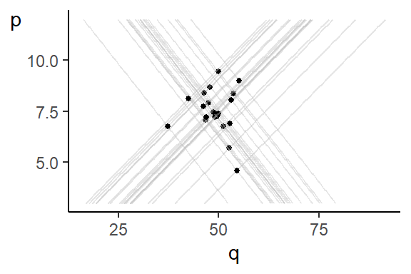
The issue here is that both prices and quantity are simultaneously determined, so both are endogenous. Price, in particular, is not exogenous: all variation in the data come from both demand and supply shocks. Both demand and supply shocks shift demand/supply functions. Shifts in either demand or supply function changes both quantity and price. The regressor (price) is therefore correlated with the regression noise term.
Now suppose there is some observable variable \(r_t\) that shifts the supply function but not the demand function. That is, the market is represented by \[ \begin{aligned} Q^d &= \delta_0 + \delta_1 P + \epsilon^d \hspace{1cm} &(\text{Demand Eq } \delta_1 < 0) \\ Q^s &= \alpha_0 + \alpha_1 P + \alpha_2r + \epsilon^s \hspace{0.5cm} &(\text{Supply Eq } \alpha_1 > 0) \\ Q^s &= Q^d \hspace{2.5cm} &(\text{Market Clearing}) \end{aligned} \] where \(\alpha_2 \neq 0\) and \(r\) are uncorrelated with the demand shocks. Imagine further that we can “shut down” the demand and supply shocks, allowing only \(r\) to change. Then only the supply curve changes (as \(r\) changes) and intersections of demand and supply maps out the demand function.
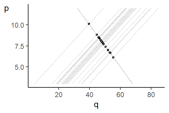
This illustrates the point that variation in \(r\) helps to “identify” the demand function. The problem is that in reality we cannot “shut down” the demand shocks, so how do we isolate variation in \(P\) due to \(r\) only? The two stage least squares perspective show that we can do so by regressing \(P_i\) on \(r_i\), and then regress \(Q_i\) on fitted \(P_i\), i.e., \(\hat{P}_i\), instead of \(P_i\), since \(\hat{P}_i\) contains variation in \(Y_i\) due to \(r_i\) only. We say that we use \(r_i\) as “instrument” to identify demand function.
There are a few important points to note. First, \(iv/2sls/mm\) estimators are in general biased estimators: \[ \begin{aligned} \hat{\beta}_1^{iv} &= \beta_1 + \frac{\sum_{i=1}^n(Z_i - \overline{Z})\epsilon_i} {\sum_{i=1}^n(Z_i - \overline{Z})X_i} \\[1.5ex] E(\hat{\beta}_1^{iv} \mid X_1, \dots, X_n, Z_1, \dots, Z_n) &= \beta_1 + \frac{\sum_{i=1}^n(Z_i - \overline{Z})E(\epsilon_i \mid X_1, \dots, X_n, Z_1, \dots, Z_n)} {\sum_{i=1}^n(Z_i - \overline{Z})X_i} \end{aligned} \] but since \(\epsilon\) is correlated with \(X\), \(E(\epsilon_i \mid X_1, \dots, X_n, Z_1, \dots, Z_n)\) will be some function of \(X_i\), \(i=1, \dots, n\), and cannot come out of the summation. Despite the bias, the \(mm/tsls/iv\) estimator is consistent. The bias disappears, and the estimator converges in probability to the desired parameter value.
Second, there is a trade-off in obtaining the consistency, which is that in general our estimators will be less precise (have larger standard errors). Suppose \(\mathit{Var}(\epsilon \mid X, Z) = \sigma^2\), then \(\mathit{Var}(\epsilon_i \mid X_1, \dots, X_n, Z_1, \dots, Z_n) = \sigma^2\) and we have \[ \begin{aligned} \mathit{Var}(\hat{\beta}_1^{iv} \mid \dots) &= \frac{\sum_{i=1}^n(Z_i - \overline{Z})^2Var(\epsilon_i\mid \dots)} {(\sum_{i=1}^n(Z_i - \overline{Z})(X_i-\overline{X}))^2} \\[1.5ex] &= \frac{\sigma^2\sum_{i=1}^n(Z_i - \overline{Z})^2} {(\sum_{i=1}^n(Z_i - \overline{Z})(X_i-\overline{X}))^2} \\[1ex] &= \frac{\sigma^2} {\sum_{i=1}^n(X_i - \overline{X})^2\left(\dfrac{(\sum_{i=1}^n(Z_i - \overline{Z})(X_i-\overline{X}))^2} {\sum_{i=1}^n(Z_i - \overline{Z})^2\sum_{i=1}^n(X_i - \overline{X})^2} \right)} \\[1ex] &= \frac{\sigma^2} {R_{X|Z}^2\sum_{i=1}^n(X_i - \overline{X})^2} \end{aligned} \] where \(R_{X|Z}^2\) is the \(R^2\) from the regression of \(X_i\) on \(Z_i\). Since \(0 \leq R_{X|Z}^2 < 1\), \(\mathit{Var}(\hat{\beta}_1^{iv} \mid \dots)\) is larger than the variance of the OLS estimator. The two are the same if \(R_{X|Z} = 1\), but in this case, \(X_i\) and \(Z_i\) are perfectly correlated, and \(Z_i\) must also be endogenous, so not a valid instrument. (If \(X\) is correlated with \(\epsilon\), and \(Z\) is not correlated with \(\epsilon\), then \(Z\) cannot be perfectly correlated with \(X\).)
The problem with IVs is that often, the correlation between \(X\) and \(Z\) is too low. If \(R_{X|Z}^2\) is near zero, then the variance of the IV estimator will be very large, to the point that the IV estimator may be effectively useless. Furthermore, although technically consistent, in finite samples the estimator may behave quite poorly. Recall the consistency proof: \[ \hat{\beta}_1^{mm} = \beta_1 + \frac{\sum_{i=1}^n(Z_i - \overline{Z})\epsilon_i} {\sum_{i=1}^n(Z_i - \overline{Z})X_i} \;\overset{p}{\longrightarrow}\; \beta_1 + \frac{\mathit{Cov}(Z, \epsilon)}{{\mathit{Cov}(Z, X)}} = \beta_1 \] In finite samples, \(\mathit{Cov}(Z, \epsilon)\) is unlikely to be exactly zero. If \(\mathit{Cov}(Z, X)\) is close to zero in population, the sample covariance between \(Z_i\) and \(X_i\) is likely to be small, resulting in a large finite sample bias. We call an instrumental variable that is poorly correlated with the endogenous regressor a “weak instrument”.
To estimate \(\sigma^2\), use: \[ \widehat{\sigma_{iv}^2} = \dfrac{1}{n-2}\sum_{i=1}^n\widehat{\epsilon}_{i, iv}^2 \] where \(\widehat{\epsilon}_{i, iv} = Y_i - \widehat{\beta}_0^{iv} + \widehat{\beta}_1^{iv} X_i\). Note that \(\widehat{\epsilon}_{i, iv}\) uses \(X_i\) rather that \(\widehat{X}_i\). Furthermore, it is conventional to divide by \(n-2\) even though IV/MM/2SLS only has large sample justifications. For \(R^2\), use: \[ R^2 = 1 - \dfrac{\sum_{i=1}^n\widehat{\epsilon}_{i, iv}^2}{\sum_{i=1}^n (Y_i - \overline{Y})^2} \] which will be less than the OLS \(R^2\).
Example 8.2 We illustrate the theory with a simulated version of the demand and supply example. Suppose \[ \begin{aligned} Q_i^d &= 8 - 2 P_i + \epsilon_i^d \hspace{1cm} &(\text{Demand Eq } \delta_1 < 0) \\ Q_i^s &= -2 + 2P_i + 0.8r_i + \epsilon_i^s \hspace{0.5cm} &(\text{Supply Eq } \alpha_1 > 0) \\ Q_i^s &= Q_i^d \hspace{2.5cm} &(\text{Market Clearing}) \end{aligned} \] where \(r_i \sim N(3,4)\) is observed, but the \(e_i^d \sim N(0,1)\) and \(e_i^s \sim N(0,1)\) are not. The code below simulates and plots 100 observations of the observed equilibrium prices and quantities.
set.seed(13)
a0 <- 8; a1 <- -2; b0 <- -2; b1 <- 2; b2 = 0.8
n <- 100; p <- seq(0.5, 4, 0.1)
pstar <- qstar <- r <- rep(0, n)
p1 <- ggplot()
for (i in 1:n){
  r[i]  <- rnorm(1,3,2)
  es <- rnorm(1,0,1); ed <- rnorm(1,0,1)
  plotdat <- tibble(
               p = p,
               qd = a0 + a1*p + ed,
               qs = b0 + b1*p + b2*r[i] + es)
  pstar[i] <- (b0 - a0)/(a1-b1) + b2*r[i]/(a1-b1) + (es-ed)/(a1-b1)
  qstar[i] <- a0 + a1*pstar[i] + ed
  p1 <- p1 + geom_line(data=plotdat, aes(x=p, y=qs), color='gray', alpha=0.3) +
    geom_line(data=plotdat, aes(x=p, y=qd), color='gray', alpha=0.3)
}
dat <- tibble(p=pstar, q=qstar)
p1 <- p1 + geom_point(data=dat, aes(x=pstar, y=qstar), size = 1, color="blue") +
  ylab("q") + theme_bw()
p1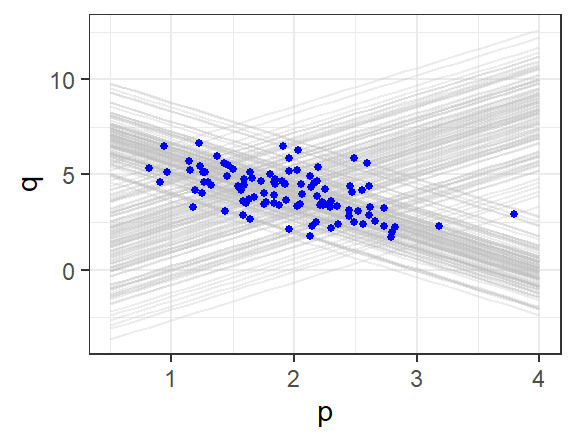
The OLS Estimates
dat <- tibble(p=pstar, q=qstar, r=r)
ddss_ols <- lm(q~p, data=dat)
summary(ddss_ols)$coefficients
Estimate Std. Error t value Pr(>|t|)
(Intercept) 6.341252 0.3660495 17.323483 1.366065e-31
p -1.175239 0.1816905 -6.468357 3.906490e-09The IV Estimates (using ivreg package, default standard errors) are
ddss_iv <- ivreg(q ~ p | r, data=dat)
ddss_coef <- summary(ddss_iv)$coef
attr(ddss_coef, "df") <- NULL
attr(ddss_coef, "nobs") <- NULL
ddss_coef
Estimate Std. Error t value Pr(>|t|)
(Intercept) 8.492688 0.5937838 14.302662 9.954936e-26
p -2.283065 0.3000241 -7.609603 1.710061e-11The IV Estimates (using ivreg package, heteroskedasticity-robust standard errors) are
coeftest(ddss_iv, vcov=vcovHC(ddss_iv, type="HC0"))
t test of coefficients:

            Estimate Std. Error t value  Pr(>|t|)
(Intercept)  8.49269    0.57835 14.6845 < 2.2e-16 ***
p           -2.28306    0.28389 -8.0421 2.063e-12 ***
---
Signif. codes:  0 '***' 0.001 '**' 0.01 '*' 0.05 '.' 0.1 ' ' 1
As expected, the IV estimate is much closer to true value of the demand elasticity parameter than OLS estimates. Default and heteroskedastic estimates for IV estimates are similar (not surprising, since data is homoskedastic), and the standard error of the IV estimator is larger than standard error of the OLS estimator.
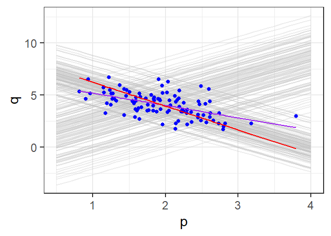
Fig. 8.4 contains plot of OLS (purple) and IV (red) estimated regression lines.
As an illustration, we manually compute below the IV estimate, with non-heteroskedasticity-robust and heteroskedasticity-robust standard errors:
y <- as.matrix(dat$q)                                #
X <- as.matrix(cbind(rep(1, length(dat$p)), dat$p))  # Assemble data
Z <- as.matrix(cbind(rep(1, length(dat$r)), dat$r))  #
b_iv <- solve(t(Z) %*% X) %*% (t(Z) %*% y)    # calculate IV estimate
# var-cov assuming homoskedasticity
y_iv_hat <- X %*% b_iv
e_iv <- y - y_iv_hat
s2 <- sum(e_iv^2) / (n-2)
var_b <- s2 * solve(t(Z) %*% X) %*% (t(Z) %*% Z) %*% solve(t(X) %*% Z)
# Robust variance-covariance
S <- matrix(c(0,0,0,0), nrow=2)
for (i in 1:n){
  zi <- matrix(Z[i,], nrow=2)
  S <- S + e_iv[i]^2 * zi %*% t(zi)
}
var_b_rb <- solve(t(Z) %*% X) %*% S %*% solve(t(X) %*% Z)

iv_coefs <- cbind(b_iv, sqrt(diag(var_b)), sqrt(diag(var_b_rb)))
colnames(iv_coefs) <- c("Estimate", "default s.e.", "robust s.e.")
rownames(iv_coefs) <- c("(Intercept)", "X")
iv_coefs
Estimate default s.e. robust s.e.
(Intercept) 8.492688 0.5937838 0.5783452
X -2.283065 0.3000241 0.2838908We have successfully replicated estimates from ivreg package.
8.2 Using Matrix Algebra
As an intermediate step towards more elaborate scenarios, which will require matrix algebra, we express the simple case from the previous sections (one endogenous regressor, one instrument, no exogenous regressors) using matrix algebra. Suppose the regression equation of interest is: \[ Y = \beta_0 + \beta_1 X_{1} + \epsilon \] where \(X_{1}\) is endogenous (correlated with the noise term). Suppose \(Z_{1}\) is correlated with \(X_{1}\) and uncorrelated with \(\epsilon\). Note that the variables previously labelled as \(X\) and \(Z\) are now labelled as \(X_1\) and \(Z_1\). The population moment conditions are: \[ E(\epsilon) = E(Y - \beta_0 - \beta_1 X_{1}) = 0 \;\;\text{ and } \;\; E(\epsilon Z_{1}) = E((Y - \beta_0 - \beta_1 X_{1})Z_{1}) = 0 \,. \] The sample moment conditions are \[ \begin{aligned} \sum_{i=1}^{n} (Y_{i} - \hat{\beta}_0^{mm} - \hat{\beta}_1^{mm} X_{i1}) = 0 \\ \sum_{i=1}^{n} (Y_{i} - \hat{\beta}_0^{mm} - \hat{\beta}_1^{mm} X_{i1})Z_{i1}= 0 \end{aligned} \] In matrix algebra, we can write this as \[ Z^\mathrm{T}(y-X\hat{\beta}^{mm}) = Z^\mathrm{T}y-Z^\mathrm{T}X\hat{\beta}^{mm} = 0 \] where \[ y = \begin{bmatrix} Y_1 \\ \vdots \\ Y_n \end{bmatrix} , \; X = \begin{bmatrix} 1 & X_{11} \\ \vdots & \vdots \\ 1 & X_{n1} \\ \end{bmatrix} , \; \varepsilon = \begin{bmatrix} \epsilon_1 \\ \vdots \\ \epsilon_n \end{bmatrix} , \; Z = \begin{bmatrix} 1 & Z_{11}\\ \vdots &\vdots \\ 1 & Z_{n1}\\ \end{bmatrix} \]
A few remarks: first, note that \(Z^\mathrm{T}X\) is \(2 \times 2\). Second, \(Z_{i1}\) correlated with \(X_{i1}\) means that \(Z^\mathrm{T}X\) is invertible. Solving the moment conditions then gives \[ \widehat{\beta}^{mm} = (Z^\mathrm{T}X)^{-1}Z^\mathrm{T}y \tag{8.10}\]
Now consider the two-stage least squares approach. In step 1, regress \(X\) on \(Z\). As \(X\) is \(n \times 2\), this means regressing each column of \(X\) on \(Z\): \[ i_n = Zb_0 + u_{*0} \;\text{ and }\; X_{*1} = Zb_1 + u_{*1} \] We can put into this one single matrix: \[ \begin{bmatrix} i_n & X_{*1} \end{bmatrix} = Z\begin{bmatrix}b_0 & b_1 \end{bmatrix} + \begin{bmatrix} u_{*0} & u_{*1} \end{bmatrix} \] or \(X = ZB + U\). We have \(\hat{B} = (Z^\mathrm{T}Z)^{-1}Z^\mathrm{T}X\). The fitted value from this step is \[ \hat{X} = Z\hat{B} = Z(Z^\mathrm{T}Z)^{-1}Z^\mathrm{T}X\,. \]
In step 2, regress \(y\) on \(\hat{X}\), which gives \[ \begin{aligned} \widehat{\beta}^{2sls} &= (\hat{X}^\mathrm{T}\hat{X})^{-1}\hat{X}^\mathrm{T}y \\[1ex] &= (X^\mathrm{T}Z(Z^\mathrm{T}Z)^{-1}Z^\mathrm{T}Z(Z^\mathrm{T}Z)^{-1}Z^\mathrm{T}X)^{-1} X^\mathrm{T}Z(Z^\mathrm{T}Z)^{-1}Z^\mathrm{T}y \\[1ex] &= (X^\mathrm{T}Z(Z^\mathrm{T}Z)^{-1}Z^\mathrm{T}X)^{-1} X^\mathrm{T}Z(Z^\mathrm{T}Z)^{-1}Z^\mathrm{T}y \\[1ex] &= (Z^\mathrm{T}X)^{-1}(Z^\mathrm{T}Z)(X^\mathrm{T}Z)^{-1}X^\mathrm{T}Z(Z^\mathrm{T}Z)^{-1}Z^\mathrm{T}y \\[1ex] &= (Z^\mathrm{T}X)^{-1}Z^\mathrm{T}y\,. \end{aligned} \tag{8.11}\] As expected, we get the same formula, which we will refer to as the IV estimator \[ \beta^{iv} = (Z^\mathrm{T}X)^{-1}Z^\mathrm{T}y\,. \tag{8.12}\]
Showing consistency is straightforward: \[
\begin{aligned}
\hat{\beta}^{iv}
&= (Z^\mathrm{T}X)^{-1}Z^\mathrm{T}y
= (Z^\mathrm{T}X)^{-1}Z^\mathrm{T}(X\beta + \epsilon) \\[1ex]
&= \beta + (Z^\mathrm{T}X)^{-1}Z^\mathrm{T}\epsilon \\[1ex]
&= \beta + (\tfrac{1}{n}Z^\mathrm{T}X)^{-1}(\tfrac{1}{n}Z^\mathrm{T}\epsilon) \overset{p}\longrightarrow \beta
\end{aligned}
\]
since \(\tfrac{1}{n}Z^\mathrm{T}\epsilon \overset{p}\rightarrow 0_{2 \times 1}\) and we assume \(\tfrac{1}{n}Z^\mathrm{T}X\) converges to a non-singular matrix. We omit the arguments for asymptotic normality.
For asymptotically valid variance-covariance matrices, we have for homoskedastic errors: \[ \widehat{\mathit{Var}}(\hat\beta_{iv}) = \widehat{\sigma^2}(Z^\mathrm{T}X)^{-1}Z^\mathrm{T}Z(X^\mathrm{T}Z)^{-1} \tag{8.13}\] where \(\widehat{\sigma^2}\) is as previously defined. The heteroskedasticity-robust version is: \[ \widehat{\mathit{Var}}_{HC0}(\hat\beta_{iv}) = (Z^\mathrm{T}X)^{-1} \left(\sum\limits_{i=1}^n \widehat{\epsilon}_{i, iv}^2 Z_{i*}^\mathrm{T} Z_{i*} \right) (X^\mathrm{T}Z)^{-1} \tag{8.14}\] where \(Z_{i*}\) are the \(i\)-rows of \(Z\)
8.3 Generalization
Suppose now that in your regression you have multiple regressors, some of which are correlated with the error term (i.e., some are endogenous) and some are not correlated with the error term. That is, you have both endogenous and exogenous regressors. We allow for the possibility that there are more instrument variables than there are endogenous variables. To start, we assume 1 exogenous regressor, 1 endogenous regressor, and 2 valid instruments for endogenous regressor: \[ Y = \beta_0 + \beta_1 X_{1}^k + \beta_2 X_{2}^g + \epsilon \] where \(X_{1}^k\) is exogenous (not correlated with the noise term), \(X_{2}^g\) is endogenous (correlated with the noise term), and there exists \(Z_{2}\) and \(Z_{3}\) both correlated with \(X_{2}^g\) and uncorrelated with \(\epsilon\).
We must have at least as many instruments as we do endogenous variables. When we have more instruments than endogenous variables, we say we have “overidentification”. If we have the same number of instruments as we do endogenous variables, we say we have “just-identification”.
8.3.1 Method of Moments Approach:
In our specific example (1 exog, 1 endog, 2 instruments), the population satisfies \(E(\epsilon) = 0\), \(\mathit{Cov}(X_1^k, \epsilon)=0\), \(\mathit{Cov}(Z_2, \epsilon)=0\), \(\mathit{Cov}(Z_3, \epsilon)=0\). That is, \[ \begin{aligned} E(\epsilon) &= E(Y - \beta_0 - \beta_1 X_{1}^k - \beta_2 X_{2}^g) = 0 \\[1ex] E(\epsilon X_{1}^k) &= E((Y - \beta_0 - \beta_1 X_{1}^k - \beta_2 X_{2}^g)X_{1}^k) = 0 \\[1ex] E(\epsilon Z_{2}) &= E((Y - \beta_0 - \beta_1 X_{1}^k - \beta_2 X_{2}^g)Z_{2}) = 0 \\[1ex] E(\epsilon Z_{3}) &= E((Y - \beta_0 - \beta_1 X_{1}^k - \beta_2 X_{2}^g)Z_{3}) = 0 \end{aligned} \] Suppose we have a representative iid sample \(\{X_{i1}^k, X_{i2}^g, Z_{i2}, Z_{i3}, Y_i\}_{1=i}^n\) from the population. The sample moments corresponding to the population moments are \[ \begin{aligned} \frac{1}{n}\sum_{i=1}^n \hat\epsilon_i^{mm} &= \frac{1}{n}\sum_{i=1}^n (Y_{i} - \hat{\beta}_0^{mm} - \hat{\beta}_1^{mm} X_{i1}^k - \hat{\beta}_2^{mm} X_{i2}^g) = 0 \\ \frac{1}{n} \sum_{i=1}^n \hat\epsilon_i^{mm} X_{i1}^k &= \frac{1}{n}\sum_{i=1}^n((Y_{i} - \hat{\beta}_0^{mm} - \hat{\beta}_1^{mm} X_{i1}^k - \hat{\beta}_2^{mm} X_{i2}^g)X_{i1}^k) = 0 \\ \frac{1}{n}\sum_{i=1}^n \hat\epsilon_i^{mm}Z_{i2} &= \frac{1}{n}\sum_{i=1}^n((Y_{i} - \hat{\beta}_0^{mm} - \hat{\beta}_1^{mm} X_{i1}^k - \hat{\beta}_2^{mm} X_{i2}^g)Z_{i2}) = 0 \\ \frac{1}{n}\sum_{i=1}^n \hat\epsilon_i^{mm}Z_{i3} &= \frac{1}{n}\sum_{i=1}^n((Y_{i} - \hat{\beta}_0^{mm} - \hat{\beta}_1^{mm} X_{i1}^k - \hat{\beta}_2^{mm} X_{i2}^g)Z_{i3}) = 0 \end{aligned} \]
We want to “solve” these sample moments for \(\hat{\beta}_0^{mm}\), \(\hat{\beta}_1^{mm}\), \(\hat{\beta}_2^{mm}\), but we have 4 equations in 3 unknowns, so the equations cannot be solved exactly. Instead, we choose \(\hat{\beta}_0^{mm}\), \(\hat{\beta}_1^{mm}\), \(\hat{\beta}_2^{mm}\) to make “LHS as close to zero” as possible. In particular, choose \(\hat{\beta}_0^{mm}\), \(\hat{\beta}_1^{mm}\), \(\hat{\beta}_2^{mm}\) to minimize the sum of squared moments: \[ \left(\sum_{i=1}^n \hat\epsilon_i^{mm}\right)^2 + \left(\sum_{i=1}^n \hat\epsilon_i^{mm}X_{i1}^k\right)^2 + \left(\sum_{i=1}^n \hat\epsilon_i^{mm}Z_{i2}\right)^2 + \left(\sum_{i=1}^n \hat\epsilon_i^{mm}Z_{i3}\right)^2\,. \] In matrix algebra terms, if we let \[ y = \begin{bmatrix} Y_1 \\ Y_2 \\ \vdots \\ Y_n \end{bmatrix} , \; X = \begin{bmatrix} 1 & X_{11}^k & X_{12}^g \\ 1 & X_{21}^k & X_{22}^g \\ \vdots & \vdots & \vdots \\ 1 & X_{n1}^k & X_{n2}^g \\ \end{bmatrix} , \; \hat{\beta}^{mm} = \begin{bmatrix} \hat{\beta}_0^{mm} \\[0.5ex] \hat{\beta}_1^{mm} \\[0.5ex] \hat{\beta}_2^{mm} \end{bmatrix} , \; Z = \begin{bmatrix} 1 & X_{11}^k & Z_{12} & Z_{13}\\ 1 & X_{21}^k & Z_{22} & Z_{23}\\ \vdots & \vdots & \vdots &\vdots \\ 1 & X_{n1}^k & Z_{n2} & Z_{n3}\\ \end{bmatrix} \] then sample moments (dropping the \(1/n\)) are: \[ \underbrace{\phantom{(}Z^\mathrm{T}}_{4 \times n}\underbrace{(y-X\hat{\beta}^{mm})}_{n \times 1} = \underbrace{\phantom{(}Z^\mathrm{T}}_{4 \times n} \underbrace{y}_{n \times 1} - \underbrace{\phantom{(}Z^\mathrm{T}}_{4 \times n} \underbrace{X}_{n \times 3} \underbrace{\phantom{(}\hat{\beta}^{mm}}_{3 \times 1} = \underbrace{0}_{4 \times 1}\,. \]
We choose \(\hat{\beta}_0^{mm}\), \(\hat{\beta}_1^{mm}\), \(\hat{\beta}_2^{mm}\) to minimize the “sum of squared moments” \[ \begin{aligned} &\underbrace{(Z^\mathrm{T}y-Z^\mathrm{T}X\hat{\beta})^\mathrm{T}}_{1 \times 4} \underbrace{(Z^\mathrm{T}y-Z^\mathrm{T}X\hat{\beta})}_{4 \times 1} \\[1ex] = \;\;&y^\mathrm{T}ZZ^\mathrm{T}y - 2\hat{\beta}^\mathrm{T}X^\mathrm{T}ZZ^\mathrm{T}y + \hat{\beta}^\mathrm{T}X^\mathrm{T}ZZ^\mathrm{T}X\hat{\beta} \end{aligned} \tag{8.15}\] Minimizing this gives \[ \hat{\beta}^{mm} = (X^\mathrm{T}ZZ^\mathrm{T}X)^{-1}X^\mathrm{T}ZZ^\mathrm{T}y \tag{8.16}\] which requires that the \(3 \times 3\) matrix \(X^\mathrm{T}ZZ^\mathrm{T}X\) be invertible.
To show consistency of the MM estimator: \[ \begin{aligned} \hat{\beta}^{mm} &= (X^\mathrm{T}ZZ^\mathrm{T}X)^{-1}X^\mathrm{T}ZZ^\mathrm{T}y \\[1ex] &= (X^\mathrm{T}ZZ^\mathrm{T}X)^{-1}X^\mathrm{T}ZZ^\mathrm{T}(X\beta + \epsilon) \\[1ex] &= (X^\mathrm{T}ZZ^\mathrm{T}X)^{-1}X^\mathrm{T}ZZ^\mathrm{T}X\beta + (X^\mathrm{T}ZZ^\mathrm{T}X)^{-1}X^\mathrm{T}ZZ^\mathrm{T}\epsilon \\[1ex] &= \beta + ((\tfrac{1}{n}X^\mathrm{T}Z)((\tfrac{1}{n}Z^\mathrm{T}X))^{-1}((\tfrac{1}{n}X^\mathrm{T}Z)(\tfrac{1}{n}Z^\mathrm{T}\epsilon) \;\;\overset{p}{\longrightarrow} \beta \end{aligned} \] which requires that \(\tfrac{1}{n}Z^\mathrm{T}\epsilon \overset{p}{\rightarrow} 0_{4 \times 1}\) and \(\tfrac{1}{n}Z^\mathrm{T}X \overset{p}{\rightarrow} \Sigma_{ZX}\) full column rank. The variance-covariance matrix under homoskedasticity is: \[ \widehat{\mathit{Var}}(\hat{\beta}^{mm}) = \sigma^2(X^\mathrm{T}ZZ^\mathrm{T}X)^{-1}X^\mathrm{T}Z(Z^\mathrm{T}Z)Z^\mathrm{T}X(X^\mathrm{T}ZZ^\mathrm{T}X)^{-1} \] Estimate \(\sigma^2\) with \(\widetilde{\sigma^2} = \dfrac{1}{n}\sum\limits_{i=1}^n \hat\epsilon_{i, iv}^2\). The heteroskedasticity-robust version is \[ \widehat{\mathit{Var}}(\hat{\beta}^{mm}) = (X^\mathrm{T}ZZ^\mathrm{T}X)^{-1} X^\mathrm{T}Z \left(\sum_{i=1}^n\hat\epsilon_{i, iv}^2Z_{i*}^\mathrm{T}Z_{i*}^{\phantom{T}}\right) Z^\mathrm{T}X (X^\mathrm{T}ZZ^\mathrm{T}X)^{-1}\,. \]
What happens if we apply these formulas to the just-identified case, where the number of endogenous is equal to the number of instruments? For instance, suppose in our example that we only have \(Z_2\) to instrument for \(X_2^g\). Then \(Z^\mathrm{T}X\) is square \(3 \times 3\), and we get \[
\begin{aligned}
\hat{\beta}_{mm}
&= (X^\mathrm{T}ZZ^\mathrm{T}X)^{-1}X^\mathrm{T}ZZ^\mathrm{T}y
= (Z^\mathrm{T}X)^{-1} (X^\mathrm{T}Z)^{-1}X^\mathrm{T}ZZ^\mathrm{T}y \\[1ex]
&= (Z^\mathrm{T}X)^{-1}Z^\mathrm{T}y\,.
\end{aligned}
\] The corresponding variance-covariance matrices, under homoskedasticity, reduces to:
\[
\widehat{\mathit{Var}}(\hat{\beta}_{mm})
=
\widehat{\sigma^2}(Z^\mathrm{T}X)^{-1}(Z^\mathrm{T}Z)(X^\mathrm{T}Z)^{-1}\,.
\] The heteroskedasticity-robust version reduces to \[
\widehat{\mathit{Var}}(\hat{\beta}_{mm}) = (Z^\mathrm{T}X)^{-1}
\left(\sum_{i=1}^n\hat\epsilon_{i, iv}^2Z_{i*}^\mathrm{T}Z_{i*}^{\phantom{T}}\right) (X^\mathrm{T}Z)^{-1}
\] The MM estimator and its var-cov. matrices all collapse to the IV case derived in Section 8.2.
8.3.2 Two-Stage Least Squares Approach
We now consider the 2SLS approach for this example. In step 1, regress \(X\) on \(Z\). The coefficient estimates are \(\hat{B} = (Z^\mathrm{T}Z)^{-1}Z^\mathrm{T}X\) (this is a \(4 \times 3\) matrix). The fitted values are \(\hat{X} = Z(Z^\mathrm{T}Z)^{-1}Z^\mathrm{T}X\).
The matrix of fitted values is \(n \times 3\) in size. The first column is a vector of 1’s, the second column is \(X_{i1}^{k}\), and the third column is \(\hat{X}_{i2}^{g}\) obtained from a regression of \(X_{i2}^{g}\) on intercept, \(X_{i1}^{k}\), \(Z_{i2}\) and \(Z_{i3}\). In step 2, we regress \(y\) on \(\hat{X}\), which gives \[ \begin{aligned} \hat{\beta}^{2sls} &= (\hat{X}^\mathrm{T}\hat{X})^{-1}\hat{X}^\mathrm{T}y \\ &= (X^\mathrm{T}Z(Z^\mathrm{T}Z)^{-1}Z^\mathrm{T}Z(Z^\mathrm{T}Z)^{-1}Z^\mathrm{T}X)^{-1} X^\mathrm{T}Z(Z^\mathrm{T}Z)^{-1}Z^\mathrm{T}y \\ &= (X^\mathrm{T}Z(Z^\mathrm{T}Z)^{-1}Z^\mathrm{T}X)^{-1} X^\mathrm{T}Z(Z^\mathrm{T}Z)^{-1}Z^\mathrm{T}y \;. \end{aligned} \tag{8.17}\] This requires that the \(4 \times 3\) matrix \(Z^\mathrm{T}X\) has full column rank and that \(Z\) has full column rank. Notice that the 2SLS approach gives us a different formula from what we obtained in the MM approach.
The proof of consistency is as follows: \[ \begin{aligned} \hat{\beta}^{2sls} &= (X^\mathrm{T}Z(Z^\mathrm{T}Z)^{-1}Z^\mathrm{T}X)^{-1} X^\mathrm{T}Z(Z^\mathrm{T}Z)^{-1}Z^\mathrm{T}y \\[1ex] &= (X^\mathrm{T}Z(Z^\mathrm{T}Z)^{-1}Z^\mathrm{T}X)^{-1} X^\mathrm{T}Z(Z^\mathrm{T}Z)^{-1}Z^\mathrm{T}(X\beta + \epsilon) \\[1ex] &= (X^\mathrm{T}Z(Z^\mathrm{T}Z)^{-1}Z^\mathrm{T}X)^{-1} X^\mathrm{T}Z(Z^\mathrm{T}Z)^{-1}Z^\mathrm{T}X\beta \\ &\qquad\qquad\qquad+ (X^\mathrm{T}Z(Z^\mathrm{T}Z)^{-1}Z^\mathrm{T}X)^{-1} X^\mathrm{T}Z(Z^\mathrm{T}Z)^{-1}Z^\mathrm{T}\epsilon \\[1ex] &= \beta + (X^\mathrm{T}Z(Z^\mathrm{T}Z)^{-1}Z^\mathrm{T}X)^{-1} X^\mathrm{T}Z(Z^\mathrm{T}Z)^{-1}Z^\mathrm{T}\epsilon \\[1ex] &= \beta + (\tfrac{1}{n}X^\mathrm{T}Z(\tfrac{1}{n}Z^\mathrm{T}Z)^{-1}\tfrac{1}{n}Z^\mathrm{T}X)^{-1} \tfrac{1}{n}X^\mathrm{T}Z(\tfrac{1}{n}Z^\mathrm{T}Z)^{-1}\tfrac{1}{n}Z^\mathrm{T}\epsilon \overset{p}{\longrightarrow} \beta \end{aligned} \]
The variance-covariance matrices are (details of proofs omitted), under homoskedasticity: \[ \widehat{\mathit{Var}}(\hat{\beta}_{2sls}) = \widehat{\sigma^2} (X^\mathrm{T}Z(Z^\mathrm{T}Z)^{-1}Z^\mathrm{T}X)^{-1} \tag{8.18}\] The heteroskedasticity-robust is \[ \begin{aligned} &\widehat{\mathit{Var}}(\hat{\beta}_{2sls}) = \\ &(X^\mathrm{T}Z(Z^\mathrm{T}Z)^{-1}Z^\mathrm{T}X)^{-1} X^\mathrm{T}Z(Z^\mathrm{T}Z)^{-1} \left[\sum_{i=1}^n\hat\epsilon_{i, iv}^2Z_{i*}^\mathrm{T}Z_{i*}^{\phantom{T}}\right] (Z^\mathrm{T}Z)^{-1}Z^\mathrm{T}X(X^\mathrm{T}Z(Z^\mathrm{T}Z)^{-1}Z^\mathrm{T}X)^{-1} \end{aligned} \tag{8.19}\]
In the just-identified case, where the number of endogenous variables is equal to the number of instruments, \(Z^\mathrm{T}X\) is square, the 2SLS estimator reduces to: \[ \begin{aligned} \hat{\beta}_{2sls} &= (X^\mathrm{T}Z(Z^\mathrm{T}Z)^{-1}Z^\mathrm{T}X)^{-1}X^\mathrm{T}Z(Z^\mathrm{T}Z)^{-1}Z^\mathrm{T}y \\[1ex] &= (Z^\mathrm{T}X)^{-1}(Z^\mathrm{T}Z)(X^\mathrm{T}Z)^{-1}X^\mathrm{T}Z(Z^\mathrm{T}Z)^{-1}Z^\mathrm{T}y = (Z^\mathrm{T}X)^{-1}Z^\mathrm{T}y \end{aligned} \] which is the same as IV estimator from Section 8.2. The variance formulas also converge to IV variance formulas.
Example 8.3 We’ll use data from earnings2019.csv to estimate the equation \[
\ln earn = \beta_0 + \beta_1 age + \beta_2 \ln tenure + \beta_3 educ + \epsilon
\] The concern is that a measure of \(ability\) is unavailable, and omitted, resulting in endogeneity of the \(educ\) variable. We assume \(age\) and \(\ln tenure\) exogenous. We assume that \(feduc\) and \(meduc\) are valid instruments. Ignoring potential endogeneity, the OLS estimates are
dat <- read_csv("data\\earnings2019.csv", show_col_types=FALSE) %>%
  mutate(ln_earn = log(earn), ln_tenure=log(tenure), const = 1)

cat("Assuming homoskedasticity (default)\n")
mdl2_ols <- lm(ln_earn ~ age + ln_tenure + educ, data=dat) # Estimate OLS
summary(mdl2_ols)$coefficients %>% round(4) # Print default coefficients and standard errors

cat("\nUsing heteroskedasticity-robust standard errors")
coeftest(mdl2_ols, vcov=vcovHC, type="HC") %>% round(4)# Robust standard errors
Assuming homoskedasticity (default)
Estimate Std. Error t value Pr(>|t|)
(Intercept) 0.9699 0.0628 15.4349 0e+00
age 0.0025 0.0008 3.3341 9e-04
ln_tenure 0.1477 0.0090 16.4018 0e+00
educ 0.1268 0.0038 33.1159 0e+00
Using heteroskedasticity-robust standard errors
t test of coefficients:
Estimate Std. Error t value Pr(>|t|)
(Intercept) 0.9699 0.0655 14.8101 <2e-16 ***
age 0.0025 0.0008 3.1315 0.0017 **
ln_tenure 0.1477 0.0092 16.0494 <2e-16 ***
educ 0.1268 0.0039 32.1078 <2e-16 ***
---
Signif. codes: 0 '***' 0.001 '**' 0.01 '*' 0.05 '.' 0.1 ' ' 1Using the formulas derived in this section, the MM estimates are as follows:
## Assemble data for MM / 2SLS
y <- dat %>% select(c(ln_earn)) %>% as.matrix()
X <- dat %>% select(c(const, age, ln_tenure, educ)) %>% as.matrix()
Z <- dat %>% select(c(const, age, ln_tenure, feduc, meduc)) %>% as.matrix()
n <- length(y)
Zcol <- dim(Z)[2]
ZTX <- t(Z) %*% X ; XTZ <- t(X) %*% Z ; ZTZ <- t(Z) %*% Z ; ZTy <- t(Z) %*% y

#--MM--
beta_MM <- solve(XTZ %*% ZTX) %*% XTZ %*% ZTy
ehat_IV <- y - X %*% beta_MM
s2hat <- sum(ehat_IV^2)/n
eZZ <- matrix(0, nrow=Zcol, ncol=Zcol)
for (i in 1:n){
  eZZ <- eZZ + ehat_IV[i]^2 * t(Z[i,,drop=F]) %*% Z[i,,drop=F]
}
vbeta_MM <-  s2hat * solve(XTZ%*%ZTX) %*% XTZ %*% ZTZ %*% ZTX %*% solve(XTZ%*%ZTX)
vbeta_MM_rob <- solve(XTZ%*%ZTX) %*% XTZ %*% eZZ %*% ZTX %*% solve(XTZ%*%ZTX)

MM_results <- cbind(estimates = beta_MM,
                    s.e. = sqrt(diag(vbeta_MM)),
                    s.e.robust = sqrt(diag(vbeta_MM_rob)))
MM_results %>% round(4)
ln_earn s.e. s.e.robust
const -1.7976 0.5844 0.5911
age 0.0096 0.0026 0.0027
ln_tenure 0.1386 0.0108 0.0111
educ 0.2991 0.0336 0.0341Using the formulas derived in this section, the 2SLS estimator is
#--2SLS--
beta_TSLS <- solve(XTZ %*% solve(ZTZ) %*% ZTX) %*% XTZ %*% solve(ZTZ) %*% ZTy
ehat_TSLS <- y - X %*% beta_TSLS
s2hat_TSLS <- sum(ehat_TSLS^2)/n
eZZ_TSLS <- matrix(0, nrow=Zcol, ncol=Zcol)
for (i in 1:n){
  eZZ_TSLS <- eZZ_TSLS + ehat_TSLS[i]^2 * t(Z[i,,drop=F]) %*% Z[i,,drop=F]
}
vbeta_TSLS <-  s2hat_TSLS * solve(XTZ %*% solve(ZTZ) %*% ZTX)
vbeta_TSLS_rob <- solve(XTZ %*% solve(ZTZ) %*% ZTX) %*% XTZ %*% solve(ZTZ) %*%
  eZZ_TSLS %*% solve(ZTZ) %*% ZTX %*% solve(XTZ %*% solve(ZTZ) %*% ZTX)

TSLS_results <- cbind(estimates = beta_TSLS,
                    s.e. = sqrt(diag(vbeta_TSLS)),
                    s.e.robust = sqrt(diag(vbeta_TSLS_rob)))
TSLS_results %>% round(4)
ln_earn s.e. s.e.robust
const -0.3843 0.1915 0.2088
age 0.0032 0.0008 0.0009
ln_tenure 0.1399 0.0096 0.0098
educ 0.2205 0.0131 0.0143We can get the 2SLS estimates from the ivreg package:
mdl2_iv <- ivreg(ln_earn ~ age + ln_tenure + educ |
                   age + ln_tenure + feduc + meduc, data=dat)
mdl2_iv_coef <- summary(mdl2_iv)$coef
attr(mdl2_iv_coef,"df")<-NULL
attr(mdl2_iv_coef,"nobs")<-NULL
mdl2_iv_coef %>% round(4)
coeftest(mdl2_iv,vcov=vcovHC(mdl2_iv,type="HC0"))  %>% round(4)
Estimate Std. Error t value Pr(>|t|)
(Intercept) -0.3843 0.1916 -2.0058 0.0449
age 0.0032 0.0008 3.9523 0.0001
ln_tenure 0.1399 0.0096 14.5964 0.0000
educ 0.2205 0.0131 16.8675 0.0000
t test of coefficients:
Estimate Std. Error t value Pr(>|t|)
(Intercept) -0.3843 0.2088 -1.8406 0.0657 .
age 0.0032 0.0009 3.7345 0.0002 ***
ln_tenure 0.1399 0.0098 14.2368 <2e-16 ***
educ 0.2205 0.0143 15.4326 <2e-16 ***
---
Signif. codes: 0 '***' 0.001 '**' 0.01 '*' 0.05 '.' 0.1 ' ' 1which validates our results computed directly from the formulas.
All formulas and results continue to apply to general case with \(K\) exogenous regressors, \(G\) endogenous regressors and \(M\) instruments, \(M \geq G\) \[ Y = \beta_0 + \beta_1 X_{1}^k + \dots + \beta_K X_{K}^k + \beta_{K+1} X_{K+1}^{g} + \dots + \beta_{K+G}X_{K+G}^{g} + \epsilon \] with instrumental variables \(Z_{1}, \dots Z_{K}, Z_{K+1}, \dots Z_{K+M}\), where \(Z_1 = X_1^k, \dots, Z_K = X_K^k\), satisfying \(cov(Z_j, \epsilon) = 0\) for all \(j = 1, \dots, K+M\). The only change is that \(Z\) is now \(n \times (K+M+1)\) and \(X\) is \(n \times (K+G+1)\).
8.4 (Optimal) Generalized Method of Moments
We now consider the generalized method of moments approach, which encompasses both the MM and 2SLS estimators. The GMM estimator minimizes weighted sum of squared moments, i.e.,
\[
\hat{\beta}_{W}^{gmm}
= \text{argmin}_{\hat{\beta}} \;\underbrace{(Z^\mathrm{T}y-Z^\mathrm{T}X\hat{\beta})^\mathrm{T}
W (Z^\mathrm{T}y-Z^\mathrm{T}X\hat{\beta})}_{\text{"}J(W)\text{"}}
\tag{8.20}\] where \(W\) is some symmetric positive-definite weight matrix (may change with \(n\) and may be data dependent). We will assume this matrix is known for the moment. The matrix \(X\) is the \(n \times K+{G}+1\) matrix of regressors (exogenous and endogenous) and \(Z\) is the \(n \times K+{M}+1\) matrix of exogenous variables (exogenous regressors and instruments).
Minimizing \(J(W)\) gives \[ \hat{\beta}_{W}^{gmm} = (X^\mathrm{T}ZWZ^\mathrm{T}X)^{-1}X^\mathrm{T}ZWZ^\mathrm{T}y \qquad \text{(Exercise!)} \tag{8.21}\] Obviously MM is GMM with \(W = I_n\) and 2SLS is GMM with \(W = (Z^\mathrm{T}Z)^{-1}\). The proof of consistency is straightforward: \[ \begin{aligned} \hat{\beta}_{W}^{gmm} &= (X^\mathrm{T}ZWZ^\mathrm{T}X)^{-1}X^\mathrm{T}ZWZ^\mathrm{T}y \\[1ex] &= \beta + (X^\mathrm{T}ZWZ^\mathrm{T}X)^{-1}X^\mathrm{T}ZWZ^\mathrm{T}\epsilon \\[1ex] &= \beta + [(\tfrac{1}{n}X^\mathrm{T}Z)W(\tfrac{1}{n}Z^\mathrm{T}X)]^{-1}(\tfrac{1}{n}X^\mathrm{T}Z)W(\tfrac{1}{n}Z^\mathrm{T}\epsilon) \;\;\overset{p}{\longrightarrow}\;\; \beta \end{aligned} \] The variance-covariance matrix under homoskedasticity is: \[ \widehat{\mathit{Var}}(\hat{\beta}_{W}^{gmm}) = \widehat{\sigma^2}(X^\mathrm{T}ZWZ^\mathrm{T}X)^{-1} X^\mathrm{T}ZW (Z^\mathrm{T}Z)^{-1}WZ^\mathrm{T}X (X^\mathrm{T}ZWZ^\mathrm{T}X)^{-1} \tag{8.22}\] whereas the heteroskedasticity-robust version is \[ \begin{aligned} &\widehat{\mathit{Var}}(\hat{\beta}_{W}^{gmm}) \\ &= (X^\mathrm{T}ZWZ^\mathrm{T}X)^{-1} X^\mathrm{T}ZW \left( \sum_{i=1}^n \hat{\epsilon}_{i, gmm}^2 Z_{i*}^\mathrm{T}Z_{i*}\right) WZ^\mathrm{T}X (X^\mathrm{T}ZWZ^\mathrm{T}X)^{-1} \end{aligned} \tag{8.23}\]
The question is what the weight matrix should be? It turns out (proof omitted) that an optimal choice of weights is \[ W^* = \left(\sum_{i=1}^n \hat{\epsilon}_{i, gmm}^2 Z_{i*}^\mathrm{T}Z_{i*}\right)^{-1} \]
This is usually implemented with a two-step approach: First, compute \(\hat{\beta}_{W}^{gmm}\) for some (non-optimal) weighting matrix \(W\). The common choice is to use \(W = (Z^\mathrm{T}Z)^{-1}\), which gives the (inefficient but consistent) 2SLS estimator \(\hat{\beta}^{2sls}\), calculate \(\hat{\epsilon}_{i,2sls}\). Then calculate \(W^* = \left(\sum\limits_{i=1}^n \hat{\epsilon}_{i, 2sls}^2 Z_{i*}^\mathrm{T}Z_{i*}\right)^{-1}\). Finally, calculate the optimal GMM estimator as \[ \hat{\beta}^{gmm} = (X^\mathrm{T}Z{W^*}Z^\mathrm{T}X)^{-1}X^\mathrm{T}Z{W^*}Z^\mathrm{T}y. \tag{8.24}\] The variance-covariance matrix under homoskedasticity is \[ \widehat{\mathit{Var}}(\hat{\beta}^{gmm}) = \widehat{\sigma^2} \left(X^\mathrm{T}Z(Z^\mathrm{T}Z)^{-1}Z^\mathrm{T}X\right)^{-1} \tag{8.25}\] where \(\widehat{\sigma^2} = \dfrac{1}{n}\sum\limits_{i=1}^n \hat\epsilon_{i, gmm}^2\). The heteroskedasticity-robust version is \[ \widehat{\mathit{Var}}(\hat{\beta}^{gmm}) = \left(X^\mathrm{T}Z\left(\sum_{i=1}^N \hat{\epsilon}_{i,gmm}^2 Z_{i*}^\mathrm{T} Z_{i*}\right)^{-1}Z^\mathrm{T}X\right)^{-1} \tag{8.26}\]
The form of the variance of the optimal GMM estimator under homoskedasticity is the same as that of 2SLS, so 2SLS is as good as optimal GMM under homoskedasticity (2SLS and two-step implementation of optimal GMM are not numerically identical – they give different estimates – but both are asymptotically efficient).
Example 8.4 We calculate GMM estimates and standard errors for the earnings2019 example. We will need the following items, all of which were calculated in an earlier example: 2SLS residuals as ehat_2SLS, \(\sum\limits_{i=1}^n \hat{\epsilon}_{i, 2sls}^2 Z_{i*}^\mathrm{T}Z_{i*}\) as eZZ_TSLS, and \(X^\mathrm{T}Z\), \(Z^\mathrm{T}X\), \(Z^\mathrm{T}Z\) and \(Z^\mathrm{T}y\) as XTZ, ZTX, ZTZ and ZTy.
W <- solve(eZZ_TSLS)
beta_GMM <- solve(XTZ %*% W %*% ZTX) %*% XTZ %*% W %*% ZTy
ehat_GMM <- y - X %*% beta_GMM
s2_GMM <- mean(ehat_GMM^2)
vbeta_GMM <- s2_GMM * solve(XTZ %*% solve(ZTZ) %*% ZTX)
eZZ_GMM <- matrix(0, nrow=Zcol, ncol=Zcol)
for (i in 1:n){
  eZZ_GMM <- eZZ_GMM + ehat_GMM[i]^2 * t(Z[i,,drop=F]) %*% Z[i,,drop=F]
}
vbeta_GMM_rob <- solve(XTZ %*% solve(eZZ_GMM) %*% ZTX)
# Compile results
GMM_results <- cbind(estimates = as.vector(beta_GMM),
                    s.e. = sqrt(diag(vbeta_GMM)),
                    s.e.robust = sqrt(diag(vbeta_GMM_rob)))
# Present results
GMM_results %>% round(4)
estimates s.e. s.e.robust
const -0.3690 0.1913 0.2086
age 0.0032 0.0008 0.0009
ln_tenure 0.1404 0.0096 0.0098
educ 0.2194 0.0130 0.0143The entries in the “estimates” column give the optimal GMM estimates. The standard errors given in the column “s.e.” is appropriate for opt. GMM under the assumption of homoskedasticity. Under homoskedasticity, you can either use 2SLS or Optimal GMM. They are numerically different, but both are consistent and asymptotically efficient. Under heteroskedasticity, optimal GMM is asymptotically more efficient, but you should use the standard errors under the “s.e.robust” column. In this example, there is not much difference between the 2SLS and GMM standard errors.
In the code below, we use the GMM package to obtain optimal GMM with heteroskedasticity-robust standard errors.
GMM_results_pkg <- gmm(
  ln_earn ~ age + ln_tenure + educ, ~ age + ln_tenure + feduc + meduc,
  data = dat, wmatrix = "optimal", vcov = "MDS", type = "twoStep")
summary(GMM_results_pkg)$coef[,1:2] %>% round(4)
Estimate Std. Error
(Intercept) -0.3690 0.2086
age 0.0032 0.0009
ln_tenure 0.1404 0.0098
educ 0.2194 0.01438.5 GMM Inference
8.5.1 Testing Linear Restrictions
We can do the usual \(t\) and \(F\) tests after GMM estimation. If your regression has \(K-1\) regressors plus an intercept, then the “Wald” statistic for jointly testing \(J\) number of linear hypotheses, \(H_0: \mathcal{R}\beta = r_0\), where \(\mathcal{R}\) is \(J \times K\) and \(r_0\) is \(K\times 1\), is
\[
W = (R\hat{\beta}^{gmm}-r)^\mathrm{T}
(R\,\widehat{\mathit{Var}}(\hat{\beta}^{gmm})R^\mathrm{T})^{-1}
(R\hat{\beta}^{gmm}-r)
\; \overset{a}{\sim} \;
\chi_{(J)}^2
\] This is the usual asymptotic version of \(F\) test, using the GMM estimators and variance-covariance matrix in place of the OLS ones. Continuing with our example \[
\ln earn = \beta_0 + \beta_1 age + \beta_2 \ln tenure + \beta_3 educ + \epsilon \,,
\] we test \(H_0: \beta_1=0 \text{ and } \beta_2 = \beta_3\) or (\(\beta_2 - \beta_3 = 0\))
R = matrix(c(0,1,0,0,0,0,1,-1), nrow=2, byrow=TRUE)
r = matrix(c(0,0), ncol=1)
b = beta_GMM
V = vbeta_GMM_rob
F_stat = t(R %*% b-r) %*% solve(R %*% V %*% t(R)) %*% (R %*% b-r)
cat("F:",F_stat,", p-value:", 1-pchisq(F_stat,nrow(R)))
F: 23.78748 , p-value: 6.833054e-068.5.2 Testing for Weak Instruments
Weak instruments (those poorly correlated with the endogenous regressors) will result in estimators with poor finite sample properties (high variance, possibly large finite sample biases). To check for weak instruments, run the “first stage regression” (as though doing 2SLS manually), i.e.,
Regress each endogenous regressor on all exogenous regressors and instruments
Test for significance of the instruments in the first stage regressions
F-statistics should be large (on the order of 20 or so)
The “First Stage Regression” in our example is \[ educ_i = \delta_0 + \delta_1 age_i + \delta_2 \ln tenure_i + \delta_3 feduc_i + \delta_4 meduc_i \] and the hypothesis of invalid instrument is \(H_0: \delta_3 = \delta_4 = 0\). We test this in the code below:
mdl_firststage <- lm(educ ~ age+ln_tenure+feduc+meduc, data=dat)
linearHypothesis(mdl_firststage, c('feduc=0','meduc=0'),
                 vcov=vcovHC(mdl_firststage,type="HC1"))
Linear hypothesis test:
feduc = 0
meduc = 0

Model 1: restricted model
Model 2: educ ~ age + ln_tenure + feduc + meduc

Note: Coefficient covariance matrix supplied.

  Res.Df Df      F    Pr(>F)
1   4943
2   4941  2 252.69 < 2.2e-16 ***
---
Signif. codes:  0 '***' 0.001 '**' 0.01 '*' 0.05 '.' 0.1 ' ' 1
It appears that \(feduc_i\) and \(meduc_i\) are not weak instruments.
8.5.3 Tests of Overidentifying Restrictions
Recall that the
GMM objective function is: \(J(W) = (Z^\mathrm{T}y-Z^\mathrm{T}X\hat{\beta})^\mathrm{T}W (Z^\mathrm{T}y-Z^\mathrm{T}X\hat{\beta})\)
General GMM estimator is: \(\hat{\beta}_{W}^{gmm} = (X^\mathrm{T}ZWZ^\mathrm{T}X)^{-1}X^\mathrm{T}ZWZ^\mathrm{T}y\)
If \(Z^\mathrm{T}X\) is square (the just-identified case) and invertible, then the GMM estimator reduces to \(\hat{\beta}_{W}^{gmm}=(Z^\mathrm{T}X)^{-1}Z^\mathrm{T}y\). This, of course, is just the MM/2SLS/IV estimator. The objective function becomes: \[ J(W) = (Z^\mathrm{T}y-Z^\mathrm{T}X\hat{\beta}^{gmm})^\mathrm{T}W (Z^\mathrm{T}y-Z^\mathrm{T}X\hat{\beta}^{gmm}) = 0 \] since \[ Z^\mathrm{T}y-Z^\mathrm{T}X\hat{\beta}^{gmm} = Z^\mathrm{T}y-Z^\mathrm{T}X(Z^\mathrm{T}X)^{-1}Z^\mathrm{T}y = 0\,. \]
In the over-identified case, on the other hand, we will have \(J(W) > 0\) in general. However, if moment conditions do hold, then sample moment conditions should hold approximately, and \(J(W)\) will still be close to zero. It can be shown, in that case, that \[ J \overset{a}{\sim} \chi^2{(M-G)} \] \(M-G\) is the number of “overidentifying restrictions” (number of excess instruments). This is the “test of overidentified restrictions” or \(J\)-test. A significant \(J\)-stat indicates that one or more of the moment conditions do not hold, perhaps one (or more) of the presumed exogenous regressors is actually endogenous, or perhaps one of the instruments is not exogenous, or some combination of these situations.
In our example we have one extra moment restriction so we can carry out the J-test:
J <- t(ZTy - ZTX %*% beta_GMM) %*% solve(eZZ_GMM) %*% (ZTy - ZTX %*% beta_GMM)
Jpval <- 1-pchisq(J,ncol(Z)-ncol(X))
cat("J-stat:", J, "   p-value:", Jpval)
J-stat: 8.168 p-value: 0.004263589The J-statistic indicates some misspecification
8.6 Testing Endogeneity
If we have valid instruments, we can test if one or more (or all) of the endogenous regressors can be treated as exogenous. In the regression \(Y = X\beta+\epsilon\) suppose \[ \begin{aligned} X &= \begin{bmatrix} 1_n & X_{*1}^k & \dots & X_{*K}^k & X_{*,K+1}^g & \dots & X_{*,K+G}^g \end{bmatrix} \\[1ex] Z &= \begin{bmatrix} 1_n & X_{*1}^k & \dots & X_{*K}^k & Z_{*,K+1} & \dots & Z_{*, K+M} \end{bmatrix} \end{aligned} \] The population moment conditions are \(E(Z^\mathrm{T}\epsilon)=0\). If \(X_{K+1}^g\) is in fact not endogenous, we can add it to the vector \(Z\), i.e., \[ \tilde{Z} = \begin{bmatrix} 1_n & X_{*1}^k & \dots & X_{*K}^k & X_{*,K+1}^g & Z_{*,K+1} & \dots & Z_{*,K+M} \end{bmatrix} \] and the moment condition \(E(\tilde{Z}^\mathrm{T}\epsilon)=0\) will still hold. The idea of the test then is
Estimate the regression equation using instrument set \(Z\), get \(J_{Z}\)
Estimate the regression equation using instrument set \(\tilde{Z}\), get \(J_{\tilde{Z}}\)
If in fact \(X_{K+1}^g\) is exogenous, then both \(J\)-statistics should be close in value (with \(J_{\tilde{Z}}\) larger than \(J_{Z}\) since more moment conditions are involved when using \(\tilde{Z}\)). If \(X_{K+1}^g\) is in fact not exogenous, then there should be significant difference between \(J_{Z}\) and \(J_{\tilde{Z}}\).
Under the null that \(X_{K+1,i}^g\) is exogenous, the “difference-in-\(J\)” statistic is \[ C = J_{\tilde{Z}} - J_{Z} \;\overset{a}{\sim}\; \chi^2(Q) \] where \(Q\) is the nunmber of endogenous variables being tested for exogeneity (here \(Q=1\)).
We continue with our example, and test if \(educ\) can be treated as exogenous. One complication is that to ensure \(C>0\), the weight matrix used in computing \(J(Z)\) has to be the appropriate sub-matrix of the weight matrix used in computing \(J(\tilde{Z})\). This is implemented in the R code below.
# C-Statistic, checking if "educ" is endogenous

#-- GMM when "educ" is exogenous
#-- set up matrices
Zr <- dat %>% select(c(const, age, ln_tenure, educ, feduc, meduc)) %>% as.matrix()
Zrcol <- dim(Zr)[2]
ZrTX <- t(Zr) %*% X ; XTZr <- t(X) %*% Zr ; ZrTZr <- t(Zr) %*% Zr ; ZrTy <- t(Zr) %*% y

#-- Get the necessary weight matrices
beta_TSLS_a <- solve(XTZr %*% solve(ZrTZr) %*% ZrTX) %*% XTZr %*% solve(ZrTZr) %*% ZrTy
ehat_TSLS_a <- y - X %*% beta_TSLS_a
eZZ_TSLS_a <- matrix(0, nrow=Zrcol, ncol=Zrcol)
for(i in 1:n){
  eZZ_TSLS_a <- eZZ_TSLS_a + ehat_TSLS_a[i]^2 * t(Zr[i,,drop=F]) %*% Zr[i,,drop=F]
}
W_a <- solve(eZZ_TSLS_a)
W_b <- W_a[-4,-4]  # fourth row and column associated with educ

#--GMM with educ exog
beta_GMM_a <- solve(XTZr %*% W_a %*% ZrTX) %*% XTZr %*% W_a %*% ZrTy
ehat_GMM_a <- y - X %*% beta_GMM_a
J_a <- t(t(Zr) %*% ehat_GMM_a) %*% W_a %*% t(Zr) %*% ehat_GMM_a

#--GMM with educ endo
beta_GMM_b <- solve(XTZ %*% W_b %*% ZTX) %*% XTZ %*% W_b %*% ZTy
ehat_GMM_b <- y - X %*% beta_GMM_b
J_b <- t(t(Z) %*% ehat_GMM_b) %*% W_b %*% t(Z) %*% ehat_GMM_b

#--Calculate C stat
C_stat <- J_a - J_b
cat("C:",C_stat,", p-value:", 1-pchisq(C_stat,ncol(Zr)-ncol(Z)))
C: 46.38576 , p-value: 9.711898e-12We soundly reject the null that \(educ\) is exogenous.
8.7 Exercises
Exercise 8.1 Suppose that the variable \(Z\) is a valid instrument for \(X\) in the regression \(Y = \beta_0 + \beta_1 X + \epsilon\). Show that \[ E(Y - \beta_0 - \beta_1 X) = 0 \text{ and } E((Y - \beta_0 - \beta_1 X)Z) = 0 \] implies \(\beta_1 = \mathit{Cov}(Z, Y) / \mathit{Cov}(Z, X)\).
Exercise 8.2 Show that \[ \hat{\beta}_{mm} = (X^\mathrm{T}ZZ^\mathrm{T}X)^{-1}X^\mathrm{T}ZZ^\mathrm{T}\,. \] by minimizing the sum of squared moments in (8.15)
(You can skip the second order conditions.)
Exercise 8.3 Show that solving the minimization problem \[ \hat{\beta}_{W}^{gmm} = \text{argmin}_{\hat{\beta}} \;\underbrace{(Z^\mathrm{T}y-Z^\mathrm{T}X\hat{\beta})^\mathrm{T} W (Z^\mathrm{T}y-Z^\mathrm{T}X\hat{\beta})}_{\text{"}J(W)\text{"}} \] produces \[ \hat{\beta}_{W}^{gmm} = (X^\mathrm{T}ZWZ^\mathrm{T}X)^{-1}X^\mathrm{T}ZWZ^\mathrm{T}y\,. \] (You can skip the second-order conditions).