library(tidyverse)
library(patchwork)
library(latex2exp)2 Probability and Statistics Review
This chapter uses the following R libraries.
Other libraries may be introduced later in the chapter.
2.1 Introduction
This chapter contains a quick review of probability and statistics. The central question in statistics is: how to learn about a population given a sample of observations from that population.
Example 2.1 (a) The population of interest may be the set of all “US non-institutional working civilians aged 16 or above in 2019”. Perhaps we wish to learn what the average hourly earnings was in this population in 2018.
(b) The population of interest may be the set of all Singapore households in 2020. Perhaps we wish to learn how many dogs SG households owned on average in 2020.
(c) Consider a machine producing a certain product. The population may be all the goods that the machine can potentially produce in its lifetime. We might be interested in the defect rate of the machine.
(d) The population of interest may be the set of outcomes of an infinite number of potential tosses of a coin. We might be interested in whether the coin is fair (if the probability of obtaining heads is 0.5).
The populations in (a) and (b) are finite (though fairly large) tangible populations, whereas (c) and (d) are intangible, effectively infinite populations.
For Example 2.1(a) suppose you select, soon after 2019, a small number (1000? 5000?) of individuals from this population and ask each person sampled how much they earned per hour on average in 2018. Let \(X_i\) be individual \(i\)’s response. You calculate \[ \overline{X} = \frac{1}{n}\sum_{i=1}^n X_i = \frac{1}{n}(X_1 + X_2 + \dots + X_n) \tag{2.1}\] where \(n\) is your sample size. You use the sample average \(\overline{X}\) as an estimate of the population average. Will your sample average be a good estimate of the population average?
Statistics uses probability theory (the concepts of random variables, probability distributions, expectations and variances, etc.) to come up with estimation rules such as (2.1) and to determine the properties of such rules. We will review some probability concepts before return to the statistical problem of estimation and hypothesis testing.
2.2 Random Variables
Let \(X\) represent the numerical outcome of an action where (i) there is a range of possible outcomes, (ii) there is randomness in terms of which outcome is obtained each time the action is taken. We call \(X\) a random variable.
Example 2.2 Each of the following describes a random variable, denoted \(X\).
(a) You randomly select a person from the population in Example 2.1(a) and let \(X\) be this persons average hourly earnings in 2019.
(b) You randomly select a household from the population in Example 2.1(b) and let \(X\) be the number of dogs in this household.
(c) You take a product produced by the machine in Example 2.1(c) and observe if it is defective, \(X=1\) if defective and \(X=0\) if not defective.
(d) You toss the coin in Example 2.1(d) and note the outcome heads or tails. You set \(X=1\) if heads and \(X=0\) if tails.
Although materially quite different, you can see that the problem of learning about the defect rate of a machine, and the probability of heads in a toss of a coin are mathematically identical.
2.3 Probability Distributions
Random outcome is not the same as arbitrary outcome. For instance, in Example 2.2(a) you are more likely to receive an answer like “$20 per hour” than an answer like “$2000 per hour”. The value of \(X\) is random, but follows some “rule” in the sense that some values or range of values are more likely than other values or ranges of values. This “rule” is summarized in the probability distribution function (pdf) of the random variable.
Example 2.3 Suppose \(X\) takes possible values \(0\) or \(1\) and that outcome \(X=1\) occurs with probability \(p\), and outcome \(X=0\) occurs with probability \(1-p\), where \(0 \leq p \leq 1\). Probabilities are defined so they are never negative, and such that total probabilities always add to 1. Then the probability distribution of \(X\) is \(f_X(x) = \Pr(X=x)\) where \(x = 0, 1\) and \[ f_X(x) = p^x(1-p)^{1-x}\,,\,\,x=0, 1\,. \tag{2.2}\] We say that \(X\) has a Bernoulli distribution with parameter \(p\), or \(X \sim \text{Bernoulli}(p)\). This pdf is useful for modelling the populations in Example 2.2(c) and (d), where in (c) \(p\) is the defect rate of the machine (hopefully very small), whereas in (d) \(p\) is the probability of obtaining heads (which we might expect to be 0.5 or close to it).
Example 2.4 The random variable \(X\) has the Poisson distribution with parameter \(\lambda>0\) if \[ f_X(x) = \Pr(X=x) = \frac{e^{-\lambda}\lambda^x}{x!}\,,\,\,x=0, 1, 2, \dots\,. \tag{2.3}\] We write \(X \sim \text{Poisson}(\lambda)\). Fig. 2.1 shows the Poisson probability distribution functions for \(\lambda=0.4\). This distribution might be a good description of the population of households in Example 2.2(b) where each bar in Fig. 2.1 represents the population proportion of households with \(x\) number of dogs.
x = 0:8
lambda = 0.4
fpois = dpois(x,lambda)
df <- data.frame(x=as.factor(x), fx=fpois)
ggplot(df, aes(x=x, y=fx)) + geom_col(width=0.2) +
  ylab("Pr(X=x)") + theme_minimal()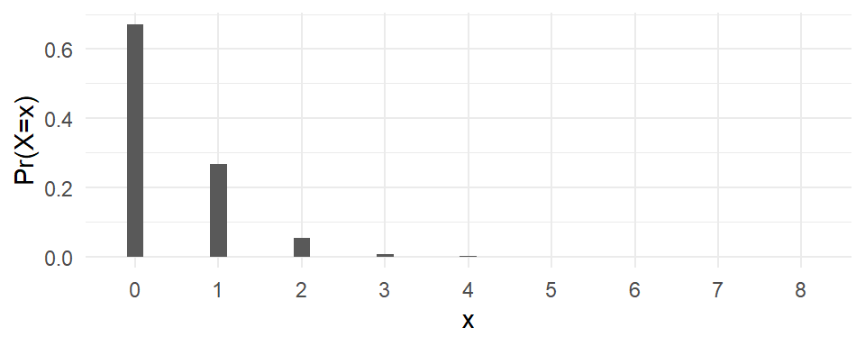
Activity: Plot the Poisson pdf for different values of \(\lambda\).
The Bernoulli and Poisson distributions have discrete ranges (distinct and separate possible values). If \(X\) has a distribution with discrete range, it is a discrete random variable. Note that the Poisson theoretically has an infinite range, though in practice the probability of a Poisson random variable taking a large integer is usually very small unless \(\lambda\) is very large.
If \(X\) takes possible values in a continuum such as the intervals \((-\infty, \infty)\), \((0, \infty)\) or \((0,1)\), then it is a continuous random variable. For continuous random variables, the probability distribution function does not give \(\Pr(X=x)\). Instead, the integral of the pdf from \(x=a\) to \(x=b\) gives the probability that an outcome of \(X\) falls between \(a\) and \(b\), \[ \Pr(a \leq X \leq b) = \int_a^b f_X(x)\,dx\,. \] Some refer to discrete distributions as probability mass functions and continuous distributions as probability density functions. I will use probability distribution function (pdf) for both.
Example 2.5 A random variable \(X\) has the normal distribution, denoted \(X \sim \mathrm{Normal}(\mu,\sigma^2)\) or \(X \sim N(\mu, \sigma^2)\), if its pdf is \[ f_{X}(x) = \frac{1}{\sigma \sqrt{2\pi}}\exp\left\{-\frac{(x - \mu)^2}{2\sigma^2}\right\} \, , \, x \in \mathbb{R}. \tag{2.4}\] The range of a normal random variable is the entire real line. The pdf of the normal distribution has the familiar symmetric bell-shape, centered at \(\mu\). The parameter \(\sigma^2\) controls how “spread out” the pdf is. The normal distribution with \(\mu=0\) and \(\sigma^2=1\) is called the standard normal distribution. The normal distribution has a special place in probability theory for reasons that will soon become clear. The normal distribution is also called the Gaussian distribution.
Fig. 2.2 displays the normal pdf with \(\mu = 1\) and \(\sigma^2 = 2\), with some regions shaded.
mu <- 1
sigma <- sqrt(2)  ## note, sigma not sigma^2
x <- seq(mu-4*sigma, mu+4*sigma, length.out = 1000)
fnorm <- dnorm(x, mean=mu, sd = sigma)
df <- data.frame(x=x, fx=fnorm)
shade1 <- subset(df, x <= -1)
shade2 <- subset(df, x >= 2 & x <= 3)
ggplot(df, aes(x=x, y=fx)) +
  geom_line(color="black") + geom_area(data = shade1, aes(x=x, y=fx), fill="grey", alpha=0.3) +
  geom_area(data = shade2, aes(x=x, y=fx), fill="grey", alpha=0.3) +
  geom_vline(xintercept = c(-1, 2, 3), linetype="dashed", color = "black")+
  scale_x_continuous(breaks=seq(floor(min(x)), ceiling(max(x)), by=1)) +
  ylab("f(x)") +  theme_minimal()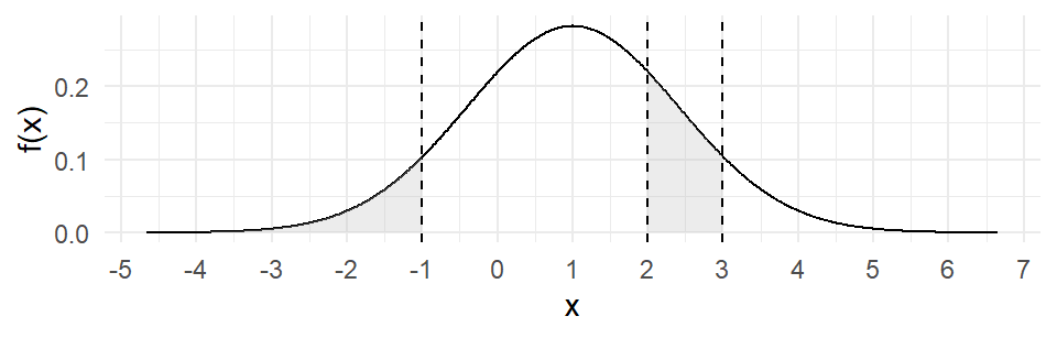
The R command pnorm(x=a, mean, sd) calculates the cumulative distribution function (cdf) of the normal distribution, defined as \[
F_X(x) = \Pr(X \leq x) = \int_{-\infty}^x f_X(u)\,du
\] for the \(\text{Normal}(\mu, \sigma)\) distribution. We can calculate the probability \(\Pr(a \leq x \leq b)\) as \[
\Pr(a \leq x \leq b) = F_X(b) - F_X(a) = \int_{-\infty}^b f_X(u)\,du - \int_{-\infty}^a f_X(u)\,du\,.
\] We have
  cat("For X ~ N(1, 2):\n")
  cat("Pr(X <= -1) =", pnorm(-1, mean=1, sd=sqrt(2)), ", ")
  cat("Pr(2 <= X <= 3) =", pnorm(3, mean=mu, sd=sigma)-pnorm(2, mean=1, sd=sqrt(2)))
For X ~ N(1, 2):
Pr(X <= -1) = 0.0786496 , Pr(2 <= X <= 3) = 0.1611005Given \(\Pr(X \leq x) = \int_{-\infty}^x f_X(u)\,du = p\), the command qnorm(p, mean, sd) finds \(x\). That is, the qnorm(p, mean, sd) function finds the \(p\)-th quantile of the normal distribution.
  cat("For X ~ N(1, 2):\n")
  cat("If Pr(X <= x) = 0.0786496, then x =", qnorm(0.0786496, mean=1, sd=sqrt(2)))
For X ~ N(1, 2):
If Pr(X <= x) = 0.0786496, then x = -1Activity: For the standard normal, find \(c\) such that (i) \(\Pr(X \leq c) = 0.025\), (ii) \(\Pr(X \geq c) = 0.025\). Find (iii) \(\Pr(X \leq -2)\) for the \(\text{Normal}(0, 4)\) distribution.
Is the normal distribution a good description of hourly earnings in the population in Example 2.2(a)? We will come to this in a moment, after discussing the idea of sampling.
If you randomly select \(n\) people from the population in Example 2.2(a) and let \(X_i\) be the average hourly earnings of individual \(i\), \(i=1, \dots, n\), then each \(X_i\) is a random variable. The set \(\{X_1, \dots, X_n\}\) is your sample. If you select these \(n\) people in such a way that each member of the population has an equal chance of getting selected, and \(n\) is large enough, then you will get a sample that is representative of the population.1 The characteristics of the sample should be similar to the characteristics of the population in terms of relative numbers of males and females, proportion of the various races, and so on. The distribution of observations in the sample should also be similar to the population distribution.
The dataset earnings2019.csv contains a random sample of almost 5000 U.S. non-institutional working civilians who had worked in 2018 (these individuals are part of the 2019 wave of the University of Michigan Panel Survey of Income Dynamics). The survey collected information regarding the surveyed individuals on variables including average hourly earnings (\(earn\)) in the previous year, number of years of schooling, age, and race. Fig. 2.3 shows histogram density estimates of the distributions of \(earn\) and \(\ln earn\). The horizontal axes in both (a) and (b) are divided into bins, and the frequency with which \(earn_i\) and \(\ln earn_i\) falls into each bin is noted. The rectangles are then scaled so that their areas sum to one.
dat1 <- read_csv("data\\earnings2019.csv", show_col_types=FALSE)
p1 <- ggplot(dat1, aes(x = earn)) +
  geom_histogram(aes(y = after_stat(density)), fill = "lightblue", color="black") +
  xlab("average earning per hour") + theme_bw()
p2 <- ggplot(dat1, aes(x = log(earn))) +
  geom_histogram(aes(y = after_stat(density)), fill = "lightblue", color="black") +
  xlab("log(average earning per hour)") + theme_bw()
p1 | p2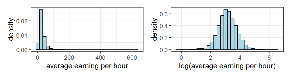
If our sample is representative of the population, then Fig. 2.3(a) strongly suggests that the normal distribution is not a reasonable distribution with which to model population earnings. Besides, average hourly earnings take only non-negative values whereas a normal distribution has range \((-\infty, \infty)\). However, Fig. 2.3(b) does suggests that the normal distribution may be a reasonable model for the population of \(\ln earn\).
2.4 Expectations
The mean or expected value of a random variable \(X\) is defined as \[ E(X) = \begin{cases} \sum_x x f_X(x) = \sum_x x \Pr(X=x) & \text{ if } X \text{ is discrete, and} \\[2ex] \int_{-\infty}^{+\infty} x f_X(x) \, dx & \text{ if } X \text{ is continuous.} \end{cases} \tag{2.5}\] The symbol \(\sum_x\) means “sum over the possible values of \(X\)”. The expected value of a random variable is therefore the weighted sum of its possible values, weighted by their corresponding probabilities.
If \(X \sim \text{Bernoulli}(p)\), then \(E(X) = 1 \cdot p + 0 \cdot (1-p) = p\).
If \(X \sim \text{Poisson}(\lambda)\), then \[ E(X) = \sum_{x=0}^\infty x \Pr(X=x) = \sum_{x=0}^\infty \frac{xe^{-\lambda}\lambda^{x}}{x!} = \lambda\,. \]
If \(X \sim \text{Normal}(\mu, \sigma^2\)), then \[ E(X) = \int_{-\infty}^{\infty} x \frac{1}{\sigma \sqrt{2\pi}}\exp\left\{-\frac{(x - \mu)^2}{2\sigma^2}\right\}\,\,dx = \mu\,. \]
For detailed proofs of these results, and other omitted proofs in this chapter, see Tay, Preve, and Baydur (2025).
2.4.1 Properties of Expectations
If \(X\) is a random variable, then \(g(X)\) is also a random variable, with expectation: \[ E(g(X)) = \begin{cases} \sum_X g(x) f_X(x) = \sum_X g(x) \Pr(X=x) & \text{ if } X \text{ is discrete, and} \\[2ex] \int_{-\infty}^{+\infty} g(x) f_X(x) \, dx & \text{ if } X \text{ is continuous.} \end{cases} \] For example, if \(X \sim \text{Bernoulli}(p)\), we have \(E(X^2) = 1^2 p + 0^2(1-p) = p\). It can also be shown that if \(X \sim \text{Poisson}(\lambda)\), then \(E(X^2) = \lambda + \lambda^2\), and if \(X \sim \text{Normal}(\mu, \sigma^2)\), then \(E(X^2) = \sigma^2 + \mu^2\).
It is straightforward to show using the properties of summation and integration that \[ E(a g(X) + b h(X)) = a E(g(X)) + b E(h(X)) \tag{2.6}\] where \(a\) and \(b\) are constants. It follows that \(E(a) = a\) for constants \(a\), and \[ E(a + b X) = a + b E(X)\,. \tag{2.7}\] We will show later than if \(X\) and \(Y\) are any two random variables, then \[ E(aX + bY) = aE(X) + bE(Y)\,. \tag{2.8}\]
2.4.2 Variance
The variance of a random variable \(X\) is its expected squared deviation from mean, i.e., \[ \mathit{Var}(X) = E((X-E(X))^2) = \begin{cases} \sum_X (x-E(X))^2 f_X(x) & \text{ if } X \text{ is discrete, and} \\[2ex] \int_{-\infty}^{+\infty} (x-E(X))^2 f_X(x) \, dx & \text{ if } X \text{ is continuous.} \end{cases} \tag{2.9}\]
The variance is a measure of the spread of the probabilities about the mean. It is sometimes referred to as the “second central moment”. The square root of the variance of \(X\) is the standard deviation of \(X\), and can be viewed as a measure of how far any given draw might be from the mean. Note that the unit of measurement of the standard deviation follows that of the variable itself. For instance, if \(X\) is measured in dollars, then the standard deviation is also measured in dollars, whereas the variance is measured in “squared dollars”.
There is another expression for the variance that is often easier to use: \[ \mathit{Var}(X) = E((X-E(X))^2) = E(X^2 - 2XE(X) + E(X)^2) = E(X^2) - E(X)^2\,. \tag{2.10}\] Using this expression for the variance, it is straightforward to show that:
If \(X \sim \text{Bernoulli}(p)\), then \(\mathit{Var}(X) = p(1-p)\).
If \(X \sim \text{Poisson}(\lambda)\), then \(\mathit{Var}(X) = \lambda\).
If \(X \sim \text{Normal}(\mu, \sigma^2)\), then \(\mathit{Var}(X) = \sigma^2\).
It follows from (2.10) that \[ \mathit{Var}(aX + b) = a^2\mathit{Var}(X)\,. \tag{2.11}\] We will show later that for any two random variables \(X\) and \(Y\), we have \[ \mathit{Var}(aX + bY) = a^2\mathit{Var}(X) + b^2\mathit{Var}(Y) + 2ab\mathit{Cov}(X,Y) \tag{2.12}\] where \(\mathit{Cov}(X,Y)\) is the covariance between the two random variables. We just note, for the moment, that if two random variables \(X\) and \(Y\) are independent (meaning that knowing the outcome of one tells you nothing about the other), then \(\mathit{Cov}(X,Y) = 0\), and \[ \mathit{Var}(aX + bY) = a^2\mathit{Var}(X) + b^2\mathit{Var}(Y)\quad\quad\textit{ NB: Only if }\mathit{Cov}(X,Y)=0. \] We will discuss independence and covariance / correlation later on in this chapter.
2.5 Jensen’s Inequality
Since \(\mathit{Var}(X) \geq 0\), (2.10) implies that \(E(X^2) \geq E(X)^2\). This is a special case of Jensen’s inequality, which says that for any random variable \(X\), we have \[ E(g(X)) \geq g(E(X)) \;\; \text{ for any convex function }\;g\,. \tag{2.13}\] The inequality is reversed if \(g\) is concave. Property (2.7) says that (2.13) holds with equality if the transformation is linear, i.e., if \(g(X) = a + bX\).
2.6 Distributions related to the normal distribution
We mention a few more distributions before discussing estimation and hypothesis testing. These distributions are all somehow related to the normal distribution.
2.6.1 Log-normal distribution
A random variable \(X\) has the log-normal distribution with parameters \(\mu\) and \(\sigma^2\) if \(\ln X \sim \text{Normal}(\mu, \sigma^2)\). Its pdf is
\[
f_X(x)
= \frac{1}{x\sigma \sqrt{2\pi}}
\exp\left\{-\frac{(\ln x - \mu)^2}{2\sigma^2}\right\} \, , \,
x \in (0,\infty)\,.
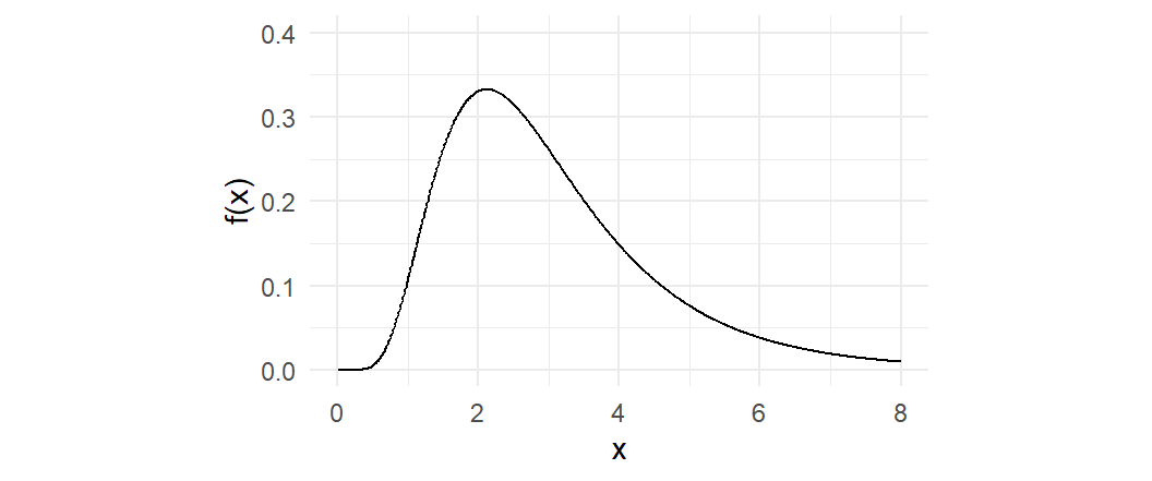
\tag{2.14}\] We write \(X \sim \text{Log-normal}(\mu, \sigma^2)\). We plot the pdf of a log-normal distribution in Fig. 2.4.
If \(X \sim \text{Log-normal}(\mu,\sigma^2)\), then \[
E(X) = \exp(\mu) \exp\left(\frac{\sigma^2}{2}\right) \;\;\text{ and }\;\;
\mathit{Var}(X) = (\exp(\sigma^2)-1)\exp(2\mu+\sigma^2)\,.
\] Another useful property of the log-normal distribution is that if \(X \sim \text{Log-normal}(\mu,\sigma^2)\), then \[
\mathit{Median}(X) = \exp(\mu)\,.
\] Since the histogram for the \(\ln(earn)\) data in our dataset earnings2019.csv appears normal, it seems like the log-normal distribution would be an appropriate model for the population distribution of \(earn\).
2.6.2 Chi-square distribution
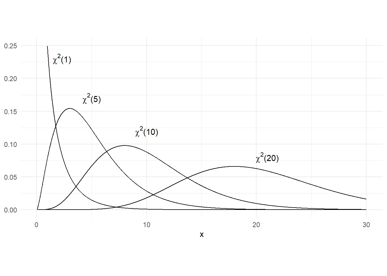
If \(X \sim \text{Normal}(0,1)\), then \(X^2\) has the “chi-square distribution with one degree of freedom”, denoted \(\chi^2(1)\). If \(X_1,X_2,\dots,X_k\) are independent standard normal random variables, then \(\sum_{i=1}^k X_i^2\) has a chi-square distribution with \(k\) degrees of freedom, denoted \(\chi^2{(k)}\). If \(X \sim \chi^2{(k)}\), then \(E(X)=k\) and \(\mathit{Var}(X)=2k\). Fig. 2.5 displays the chi-square distribution for a few different values of the “degree of freedom” parameter.
2.6.3 Student-t distribution
If \(X\) and \(W\) are independent variables with \(X \sim \text{Normal}(0,1)\) and \(W \sim \chi^2(v)\), then \[ \frac{X}{\sqrt{W / v}} \sim \mathrm{t}{(v)} \] where \(\mathrm{t}{(v)}\) denotes the student-t distribution with \(v\) degrees of freedom. A student-t random variate has zero mean, and variance \(\frac{v}{v-2}\) (the variance does not exist unless \(v>2\)). The student-t pdf is similar to that of the standard normal pdf in that it is symmetrically bell-shaped and centered about zero. However, it has fatter tails than a normal distribution. This means that a student-t random variable has greater probability of extreme realizations than a comparable normal variate. The student-t pdf has the property that it converges to the standard normal pdf as \(v \rightarrow \infty\). Fig. 2.6 shows the student-t pdf with degree-of-freedom parameter \(v=1\), \(5\), \(10\), and \(20\), and also the pdf of the standard normal. The t(1) and t(5) distributions are indicated, with the t(10) and t(20) distributions “between” the t(5) and the standard normal pdf. The following table compares the tail probabilities of the normal and the student-t distribution.
norm_vs_t_tail <- cbind(
                    pnorm(c(-2.57, -1.96, -1.64)),
                    pt(c(-2.57, -1.96, -1.64), 1),
                    pt(c(-2.57, -1.96, -1.64), 5),
                    pt(c(-2.57, -1.96, -1.64), 10),
                    pt(c(-2.57, -1.96, -1.64), 20),
                    pt(c(-2.57, -1.96, -1.64), 30))
colnames(norm_vs_t_tail) <- c("N(0,1)", "t(1)", "t(5)", "t(10)", "t(20)", "t(30)")
rownames(norm_vs_t_tail) <- c("P(X<-2.57)", "P(X<-1.96)", "P(X<-1.64)")
round(norm_vs_t_tail, 4)
N(0,1) t(1) t(5) t(10) t(20) t(30)
P(X<-2.57) 0.0051 0.1181 0.0250 0.0139 0.0091 0.0077
P(X<-1.96) 0.0250 0.1502 0.0536 0.0392 0.0320 0.0297
P(X<-1.64) 0.0505 0.1743 0.0810 0.0660 0.0583 0.0557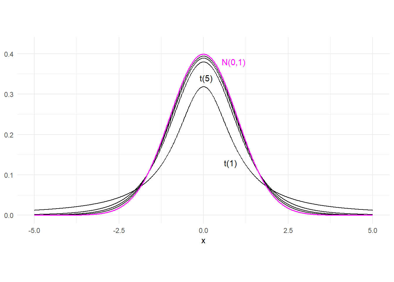
2.6.4 F distribution
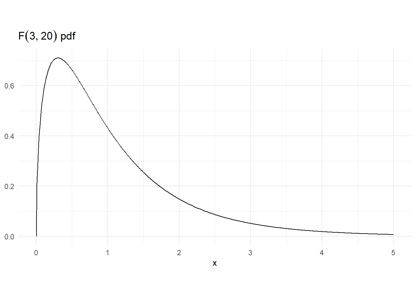
If \(W_1\) and \(W_2\) are independent chi-square random variables with degrees of freedom \(v_1\) and \(v_2\) respectively, then \[ \frac{W_1 / v_1}{W_2 / v_2} \sim F{(v_1,v_2)} \] where \(F{(v_1,v_2)}\) denotes the “F distribution with \(v_1\) and \(v_2\) degrees of freedom”. If \(X \sim F{(v_1,v_2)}\), then \[ \begin{gathered} E(X) = \frac{v_2}{v_2-2}\;\;\text{ and }\;\; \mathit{Var}(X) = 2\left(\frac{v_2}{v_2-2}\right)^2\frac{v_1+v_2-2}{v_1(v_2-4)}\;. \end{gathered} \] The F-distribution is also related to the student-t and chi-squared distributions in that
If \(X \sim \mathit{t}{(v)}\), then \(X^2 \sim F{(1,v)}\),
If \(X \sim F{(v_1,v_2)}\), then the pdf of \(v_1X\) converges to the \(\chi^2(v_1)\) pdf as \(v_2 \rightarrow \infty\).
Fig. 2.7 shows the \(F{(3,10)}\) pdf.
2.7 Estimation
In all four examples in Example 2.1, the aspect of the population that we want to learn about is the population average, or population mean. This corresponds to the expected value \(E(X)\) of the distribution that we use to model the population, where \(X\) is the random variable representing the outcome of a single draw. Our goal then is to estimate \(E(X)\).
We can begin by assuming that the population follows a certain distribution. For example, we can use the log-normal distribution as a model for the population in Example 2.1(a), or the Poisson distribution for the population in Example 2.1(b), or the binomial distribution for the populations in Example 2.1(c) and (d). For the moment, however, we shall keep things general, and merely assume that the population is characterized by the parameters \(E(X) = \mu\) and \(\mathit{Var}(X) = \sigma^2\), without assuming a specific distribution for the population.2
We assume that you have a representative i.i.d. random sample \(\{X_i\}_{i=1}^{n}\) from the population. The abbreviation “i.i.d.” means identically and independently distributed. Since we assume the sample is representative of the population, each \(X_i\) will be identically distributed, with \(E(X_i) = \mu\) and \(\mathit{Var}(X_i) = \sigma^2\) for \(i=1, \dots, n\). The “independently distributed” part means that having drawn one particular individual does not alter the probability of another individual being drawn. We will talk about independent variables in the chapter, and later in the course we will see examples of non-independent samples. For now, we will simply assume an independent sample, which implies that \(\mathit{Var}(X_i + X_j) = \mathit{Var}(X_i) + \mathit{Var}(X_j)\) for all \(i \neq j\).
Since we are trying to estimate the population mean, it seems sensible to use the sample mean as the estimator for the population mean: \[ \hat{\mu} = \frac{1}{n}\sum_{i=1}^{n} X_{i} = \overline{X}\,. \tag{2.15}\] You should think of (2.15) as a random variable. Every time you draw \(n\) observations from the population, you will get a different sample, and therefore a different sample mean. Put briefly, since the \(X_i\)’s are random, then so is their average. Being a random variable, the sample mean will have an expected value, a variance, and a distribution.
An estimator \(\widehat{\theta}\) for some parameter \(\theta\) is unbiased if \(E(\widehat{\theta}) = \theta\). It turns out that the sample mean is an unbiased estimator of the population mean: \[ E(\overline{X}) = E\left(\frac{1}{n}\sum_{i=1}^{n} X_{i}\right) = \frac{1}{n}\sum_{i=1}^{n} E(X_{i}) = \frac{1}{n} n\mu = \mu\,. \tag{2.16}\] That is, the distribution of your estimator is centered about the population mean. You can interpret this to mean that by following this estimation rule, you will not systematically over- or under-estimate your target parameter. Another way to understand unbiasedness is to imagine the following: suppose a number of statisticians were to each draw \(n\) (different) samples from the population, and each calculate the sample mean for their own sample. Each statistician will have a different sample mean. Some will overestimate the true value of \(E(X)\) whereas others will underestimate it. What unbiasedness says is that on average, the statisticians will be correct; their sample means will center about the true value of \(E(X)\).
How big of an error can we expect to make using this estimator? We can answer this question by looking at the variance of the estimator. The variance of the estimator measures the spread of the estimator’s distribution around its mean, so it is a measure of how “precise” the estimator is. Assuming we have an i.i.d. sample, we have \[ \mathit{Var}(\overline{X}) = \mathit{Var} \left( \frac{1}{n}\sum_{i=1}^n X_i \right) = \frac{1}{n^{2}}\sum_{i=1}^n \mathit{Var}(X_i) = \frac{1}{n^2} n \sigma^{2} = \frac{\sigma^{2}}{n}\,. \tag{2.17}\] The expression (2.17) tells you that the larger your sample size the smaller would your estimator variance be. A larger \(n\) means a smaller variance, so you get a more precise estimator. In your sample, some sample observations will be above the population mean, some below. When you take the average, the negative and positive errors cancel, so your overall error becomes smaller.
If you want to get a numerical estimate of the variance of the sample mean, you will have to estimate \(\sigma^2\). How do we do that? Since \[ \mathit{Var}(X) = E((X-E(X))^2) \] one obvious suggestion is to use the estimator \[ \widetilde{\sigma^2} = \frac{1}{n}\sum_{i=1}^{n} (X_i - \overline{X})^2 = \frac{1}{n}\sum_{i=1}^{n} X_i^2 - \overline{X}^2 \,. \tag{2.18}\] Then the variance of the sample mean can be estimated as \[ \widetilde{\mathit{Var}}(\overline{X}) = \frac{\widetilde{\sigma^2}}{n}\,. \] However, (2.18) turns out to be a biased estimator for \(\sigma^2\). We can show this using the fact that \[ \begin{aligned} E(X_i^2) &= \mathit{Var}(X_i) + E(X_i)^2 = \sigma^2 + \mu^2 \\[1ex] \text{and} \;\;\;E(\overline{X}^2) &= \mathit{Var}(\overline{X}) + E(\overline{X})^2 = \sigma^2/n + \mu^2\,. \end{aligned} \] We have \[ E(\widetilde{\sigma^2}) = \frac{1}{n}\sum_{i=1}^n E(X_i^2) - E(\overline{X}^2) = \sigma^2 + \mu^2 - \frac{\sigma^2}{n}-\mu^2 = \frac{n-1}{n}\sigma^2. \] The estimator (2.18) therefore systematically under-estimates the variance of the sample observations. If your sample size \(n\) is large, the bias may be negligible for all intents and purposes in which case there shouldn’t be any problem using (2.18). Nonetheless, it is easy to derive an unbiased estimator for \(\sigma^2\), namely \[ \widehat{\sigma^2} = \frac{n}{n-1}\widetilde{\sigma^2} = \frac{1}{n-1}\sum_{i=1}^n (X_i - \overline{X})^2. \tag{2.19}\] The intuition for why the divisor in (2.19) has to be \(n-1\) instead of \(n\) is that the deviations from sample mean always sum to zero. This means that there are only \(n-1\) ‘free’ deviations from sample mean. For example, given \(\sum_{i=1}^n (X_i - \overline{X})\) and the first \(n-1\) deviations \((X_i - \overline{X})\), \(i=1,2,...,n-1\), you can determine the \(n\)th deviation as \((X_i - \overline{X}) = - \sum_{i=1}^{n-1} (X_i - \overline{X})\). One “degree of freedom” was lost because we had to use the observations to compute the sample mean in order to compute the deviations from sample mean.
Once you have obtained \(\widehat{\sigma^2}\), you can replace \(\sigma^2\) in (2.17) with it. We often report the standard error for the sample mean, defined as \[ \text{s.e.}(\overline{X}) = \sqrt{\frac{\widehat{\sigma^2}}{n}}\,. \]
Example 2.6 For our average hourly earnings example, we have
cat("Estimate of 2019 average hourly earnings\n")
X = dat1$earn
n = length(X)
Xbar = sum(X)/n
s2hat = sum((X-Xbar)^2)/(n-1)
Xse = sqrt(s2hat/n)
cat("sample mean ($):", round(Xbar,2), "   ")
cat("standard error ($):", round(Xse,2))
Estimate of 2019 average hourly earnings
sample mean ($): 29.23 standard error ($): 0.37Using R built-in functions:
cat("Estimate of 2019 average hourly earnings\n")
cat("sample mean ($):", round(mean(X),2), "   ")
s2hat = var(X)
cat("standard error ($):", round(sqrt(s2hat/n),2))
Estimate of 2019 average hourly earnings
sample mean ($): 29.23 standard error ($): 0.37Example 2.7 Coins can be weighted so that one side shows more frequently than the other in random tosses of the coin. Let \(X=1\) if heads shows, and \(X=0\) if tails shows and let \(p\) be the probability of obtaining heads. Then \(X \sim \text{Binomial}(p)\). Suppose you randomly toss the coin \(n\) times and record the outcomes, giving you an i.i.d. sample \(\{X_i\}_{i=1}^n\) such that \(E(X_i)=p\) and \(\mathit{Var}(X_i) = p(1-p)\) for all \(i=1, \dots, n\). Then \(p\) can be estimated using the sample mean \(\hat{p} = \overline{X}\) which is equal to the proportion of \(1\)s in the sample. The variance of the estimator is \[ \mathit{Var}(\hat{p}) = p(1-p)/n \] which can be estimated by \[ \widehat{\mathit{Var}}(\hat{p}) = \frac{\widehat{\sigma^2}}{n} \;\;\text{ where }\; \widehat{\sigma^2}=\frac{1}{n-1}\sum_{i=1}^{n} (X_i - \overline{X})^2\,. \] We can take the square root of \(\widehat{\mathit{Var}}(\hat{p})\) to get the standard error of the estimator.
Example 2.7 is an example of estimating the population mean of an infinite conceptual population. It is nonetheless mathematically identical to the next example, where we are estimating the population mean of a finite tangible population.
Example 2.8 Suppose you are interested in estimating the proportion \(p\) of smokers in a large population of size \(N\). If \(X\) is a random draw from this population (with “smoker” = 1, “non-smoker”=0), then \(X \sim \text{Binomial}(p)\). Suppose you randomly sample \(n\) people and ask if they smoke. Suppose you have done the appropriate randomization in selecting your sample, so that you can consider your sample \(\{X_i\}_{i=1}^n\) to be a representative i.i.d. draw from the population.
As in the coin toss example, \(E(X) = p\) so an unbiased estimator for \(p\) is the sample mean, which is the proportion of smokers in your sample. You can estimate the standard error of the estimator as in the previous example.
Note that the maximum value of the variance \(\mathit{Var}(\hat{p}) = p(1-p)/n\) occurs at \(p=0.5\), i.e., for fixed \(n\), the largest value of the standard error is \[ \sqrt{\frac{0.5(1-0.5)}{n}} = \sqrt{\frac{0.25}{n}}\,. \] How many samples do you need to collect to ensure that the standard error is less than 0.01, or 1%. We have \[ \sqrt{\frac{0.25}{n}} < 0.01 \Rightarrow \frac{0.25}{n} < 0.0001 \Rightarrow n>2500\,. \] This is regardless of the size of the population.
2.8 Hypothesis Testing
To test if the population mean is equal to some specific numerical value \(\mu_0\), we check if the sample mean is “improbably far” from \(\mu_0\) when \(\mu=\mu_0\) is assumed to be true. If it is, we construe this as evidence that the null hypothesis \(H_0: E(X) = \mu_0\) is false, and reject it in favor of the alternative hypothesis \(H_A: E(X) \neq \mu_0\). But how far is “improbably far”? To provide an answer to this question, we need to derive the distribution of the sample mean when \(\mu=\mu_{0}\), and to do so we need to know the distribution of \(X\). If all you know is that \(E(X)=\mu\) and \(\mathit{Var}(X)=\sigma^2\), then you do not have enough information to derive the distribution of the sample mean.
In the case of the coin toss example, the structure of the problem does give us enough information to derive the finite sample distribution of the sample mean. Suppose \(n=2\). Then the possible values of the sample mean are \(0\), \(1/2\) and \(1\), corresponding to sample outcomes \((0,0)\), \((0,1)\) or \((1,0)\), and \((1,1)\) respectively. The corresponding probabilities are \((1-p)^2\), \(2p(1-p)\), and \(p^2\). For \(n=3\), the possible outcomes for the sample mean are:
- \(\overline{X}=0\), corresponding to outcome \((0,0,0)\), which occurs with probability \((1-p)^3\);
- \(\overline{X}=1/3\), corresponding to outcomes with 1 head out of 3 tosses. There are \(\binom{3}{1}=3\) such outcomes, so the probability is \(3p(1-p)^2\).
- \(\overline{X}=2/3\), corresponding to outcomes with 2 heads out of 3 tosses. There are \(\binom{3}{2}=3\) such outcomes, so the probability is \(3p^2(1-p)\).
- \(\overline{X}=1\), corresponding to outcome \((1,1,1)\) which occurs with probability \(p^3\).
For a sample of size \(n\), the possible values of the sample mean are \(i/n\), \(i=0,1,...,n\), each corresponding to a set of \(\binom{n}{i}\) outcomes comprising \(i\) heads out of \(n\) tosses, so the probability of obtaining a sample mean of \(i/n\) is \[ \Pr\left(\overline{X} = \frac{i}{n} \right) = \binom{n}{i}p^i(1-p)^{n-i}\,,\,\, i=0,1,2,...,n. \tag{2.20}\]
We can use (2.20) to help us decide if we should reject the hypothesis that the coin is fair.
Example 2.9 Suppose we have a sample of 20 coin tosses, and suppose that the coin is in fact fair, i.e., \(p = 0.5\). The following is the probability distribution function \(\Pr(\overline{X}= i/n)\), \(i=0,1,...,n\), of the sample mean, calculated using (2.20) with \(p=0.5\), and displayed in Fig. 2.8.
p <- 0.5
n <- 20
i <- 0:n       # i integers from 0 to 20
phat <- 0:n/n  # possible values of sample means
Pr_phat <- choose(n,i)*p^i*(1-p)^(n-i)
dim(Pr_phat) <- c(1,n+1) # make into row vector for presentation
colnames(Pr_phat) = paste0("p_hat=",i/n)
rownames(Pr_phat) = "Prob:"
noquote(format(Pr_phat, scientific=T,digits=6)) # another way to print to screen
p_hat=0 p_hat=0.05 p_hat=0.1 p_hat=0.15 p_hat=0.2 p_hat=0.25
Prob: 9.53674e-07 1.90735e-05 1.81198e-04 1.08719e-03 4.62055e-03 1.47858e-02
p_hat=0.3 p_hat=0.35 p_hat=0.4 p_hat=0.45 p_hat=0.5 p_hat=0.55
Prob: 3.69644e-02 7.39288e-02 1.20134e-01 1.60179e-01 1.76197e-01 1.60179e-01
p_hat=0.6 p_hat=0.65 p_hat=0.7 p_hat=0.75 p_hat=0.8 p_hat=0.85
Prob: 1.20134e-01 7.39288e-02 3.69644e-02 1.47858e-02 4.62055e-03 1.08719e-03
p_hat=0.9 p_hat=0.95 p_hat=1
Prob: 1.81198e-04 1.90735e-05 9.53674e-07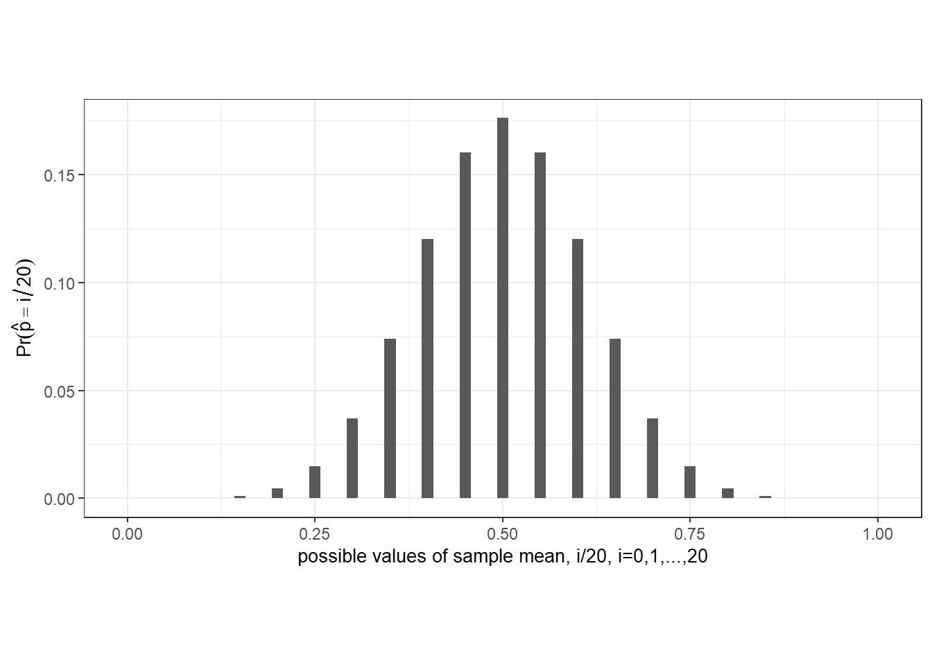
Notice that there are non-zero probabilities on every possible outcome of the sample mean. This means that any reasonable decision rule that we use to reject or not reject the null hypothesis will carry a non-zero probability of rejection even when the null hypothesis is true (we call this a “Type 1 error”). For example, suppose we use the rule “Reject \(p=0.5\) in favor of the alternative \(p \neq 0.5\) if the frequency of heads \(\hat{p}\) is less than \(0.3\) or greater than \(0.7\)”, which seems not unreasonable. We can calculate from the table above that in using this rule, there is a probability of approximately \(0.0414\) that we reject the null even though \(p\) is in fact equal to \(0.5\).
round(sum(Pr_phat[i/n<0.3])+sum(Pr_phat[i/n>0.7]),4)[1] 0.0414We can reduce the probability of Type 1 error by allowing for a larger range for \(\hat{p}\) (perhaps reject if \(\hat{p} < 0.05\) or \(\hat{p} > 0.95\)), but then the test loses power to reject a false hypothesis (i.e., the probability of failing to reject a wrong hypothesis — a “Type 2 error” — increases). In practice, researchers usually opt for rules such that the probability of an incorrect rejection of a true hypothesis is around 0.01, or 0.05, or 0.10.
What about the average hourly earnings example? Since we did not assume a specific distribution for the population, we cannot derive the distribution of the sample mean, which we need for hypothesis testing. All we know is that \(E(\overline{X}) = \mu\) and \(\mathit{Var}(X) = \sigma^2\). Had we assumed that \(X\) is normally distributed, then the sample mean \(\overline{X}\) would also be normally distributed \[ \overline{X} \sim \text{Normal}\left(\mu\,, \frac{\sigma^2}{n} \right) \;\;\text{ or }\;\; \frac{\overline{X}-\mu}{\sqrt{\sigma^2/n}} \sim \text{Normal}(0,1)\,. \] Then, replacing \(\sigma^2\) with \(\widehat{\sigma^2}\) from (2.19), it can be shown that \[ t\text{-stat} = \frac{\overline{X}-\mu}{\sqrt{\widehat{\sigma^2}/n}} \sim \text{t}(n-1)\,. \tag{2.21}\] We can then use this to do hypothesis testing. The \(t\)-stat measures the number of standard errors the sample mean is away from \(\mu\). Suppose you want to test \(H_0: \mu = 30\) vs \(H_a: \mu \neq 30\). If the null hypothesis that \(\mu = 30\) is true, then the \(t\)-stat with \(\mu\) substituted for \(30\) will have the t-distribution. The idea then is to reject the hypothesis if the sample mean is too far away from the hypothesized \(\mu = 30\). We use the following decision rule \[ \text{Reject }H_0 \;\text{ if }\;\lvert t\text{-stat} \rvert > c_{\alpha/2} \] where \(c_{\alpha/2}\) is the \(\alpha/2\)-percentile of the \(\text{t}(n-1)\) distribution. This sets the probability of rejecting the null hypothesis when it is true at \(\alpha\). The typical values of \(\alpha\) are \(0.01\), \(0.05\), \(0.10\).
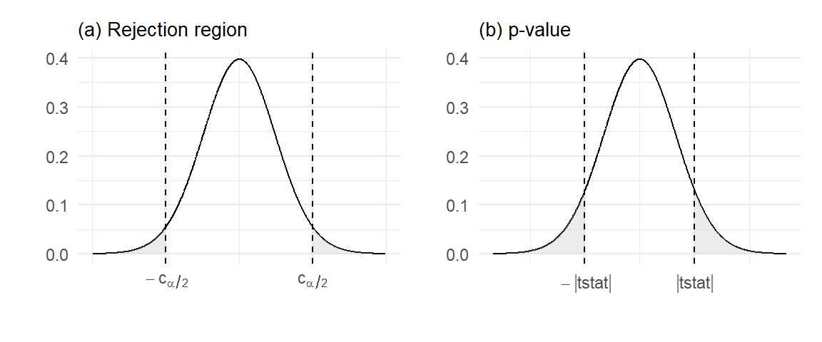
This is illustrated in Fig. 2.9(a) which plots the t-distribution. For a 0.05-significance test (where the probability of rejecting a true hypothesis is controlled at 0.05), we would choose \(c_{0.05/2}\) such that the probability in the shaded region is 0.05. For moderate values of \(n\) this is around 2, that is, we reject the hypothesis if the parameter estimate is more than twice the standard deviation away from the hypothesized value of the parameter. For large values of \(n\), the t-distribution is practically the same as the normal distribution, and \(c_{\alpha/2}\) is 1.96 for \(\alpha=0.05\).
An easier way is to report the \(p\)-value, defined as the area of the shaded region illustrated in Fig. 2.9(b), where \(t\)-stat` is the value of your \(t\)-statistic. If the \(p\)-value is greater than \(\alpha\), we do not reject the hypothesis at the \(\alpha\)-significance level. If it is smaller than \(\alpha\), we reject the hypothesis.
Example 2.10 For our average hourly earnings example, to test \(H_0: \mu=30\) vs \(H_A: \mu \neq 30\), we have
X=dat1$earn
n=length(X)
tstat = (mean(X)-30)/sqrt(var(X)/n)
pval = 2*pt(-abs(tstat), n-1)
cat("t-stat:", round(tstat, 3), "   p-val:", round(pval, 3))
t-stat: -2.087 p-val: 0.037We reject the hypothesis at 0.05 significance level, but not at 0.01 significance level.
The big question mark with the test in Example 2.10 is that the assumption that the population is normally distributed is not appropriate. It might be an appropriate assumption for \(\ln earn\) but not for \(earn\). If \(earn\) is not normally distributed, the \(t\)-stat does not have a t-distribution, and so the conclusion of the \(t\)-test might be suspect. It turns out that the test we just did is probably fine given our sample size. We explain in Section 2.9.2 the reason for this conclusion.
Notice that the sample mean remains unbiased. We did not need to make any assumptions about the specific form of the distribution in our proof that the sample mean is unbiased for the population mean. The only question is with regard to the conclusion of the hypothesis test.
2.9 Asymptotic Analysis
Asymptotic analysis refers to results that apply “in the limit”, as the sample size goes to infinity. It serves to approximate the finite sample properties of estimators if the sample size is reasonably large, and is especially helpful when the finite sample properties are unknown. We continue to focus on the sample mean, which we now denote as \(\overline{X}_n\) to indicate the sample size used to calculate it.
2.9.1 Consistency and the Law of Large Numbers
We have mentioned the desirability of larger sample sizes. For the general problem of estimating the population mean of a random variable \(X\) with mean \(\mu\) and variance \(\sigma^2\) using the sample mean, we have \(\mathit{Var}(\overline{X}_n)=\sigma^2/n \rightarrow 0\) as \(n \rightarrow \infty\). Since \(\overline{X}_n\) is unbiased, and its variance collapses to zero as the sample size goes to infinity, the estimator converges to the population mean as the sample size grows larger and larger.
The convergence of \(\overline{X}_n\) to \(\mu\) is not quite the same as the convergence of, say, the deterministic sequence \(1/n\) to zero. In the latter case, I know that if \(n\) is large enough, then \(1/n\) will definitely be within a certain distance of 0. For instance, if \(n>1000\), then \(1/n < 0.001\) for sure. In the case of \(\overline{X}_n\), which is a sequence of random variables, we cannot make such a definite claim.
The convergence concept we use for random variables is “convergence in probability”. A sequence of random variables \(Y_n\) is said to converge in probability to some value \(c\) as \(n \rightarrow \infty\) if for any \(\epsilon>0\) (no matter how small), \[ \Pr(\,|Y_n - c| > \epsilon\,) \rightarrow 0 \;\text{ as }\; n \rightarrow \infty\,. \] This allows for some probability that the distance between \(Y_n\) and \(c\) exceeds \(\epsilon\) at any sample size \(n\), but as \(n\) increases towards infinity, this probability becomes vanishingly small. We write \(\mathrm{plim}\;Y_n = c\) or \(Y_n \overset{p}{\rightarrow}c\). It can be shown that if \(E(Y_n)\) converges to \(c\) and \(\mathit{Var}(Y_n)\) converges to zero, then \(Y_n\) converges in probability to \(c\). The sample mean, therefore, converges in probability to the population mean.
In the context of parameter estimation, we say that an estimator is consistent if it converges in probability to the true value of the parameter it is estimating. The sample mean \(\overline{X}_n\) is a consistent estimator for \(\mu\) under quite general conditions. This result is known as a law of large numbers. There are several laws of large numbers, each describing a set of conditions which, if met, guarantee the consistency of the sample mean. We state one such law below:
Theorem 2.1 (Khinchine’s Weak Law of Large Numbers, WLLN) If \(\{X_i\}_{i=1}^n\) are i.i.d. with \(E(X_i) = \mu < \infty\) for all \(i\), then \[ \overline{X}_n \overset{p}{\longrightarrow} \mu\,. \]
There are other kinds of convergence concepts for sequences of random variables, but for the moment we consider only convergence in probability. The theorem above is referred to as a weak law of large numbers because the convergence concept used is convergence in probability, and there are “stronger” forms of probabilistic convergence.
The following result is used frequently:
Proposition 2.1 If \(g(.)\) is a continuous function, then \[ Y_n \overset{p}{\rightarrow} c \Rightarrow g(Y_n) \overset{p}{\rightarrow} g(c). \tag{2.22}\] That is, if \(\mathrm{plim}Y_n\) exists, and \(g(.)\) is continuous, then \(\mathrm{plim}\,g(Y_n) = g(\mathrm{plim}Y_n)\).
For example, if \(Y_n\) converges in probability to \(c\), then \(Y_n^2 \overset{p}{\rightarrow} c^2\). Result (2.22) extends to continuous functions of multiple variables. This implies that if \(Y_n \overset{p}{\rightarrow} c_y\) and \(Z_n \overset{p}{\rightarrow} c_z\), then
- \(Y_n + Z_n \overset{p}{\rightarrow} c_y + c_z\),
- \(Y_n Z_n \overset{p}{\rightarrow} c_y c_z\),
- \(Y_n / Z_n \overset{p}{\rightarrow} c_y / c_z\), as long as \(c_z\) is not zero.
Example 2.11 Suppose \(\{X_i\}_{i=1}^n\) is an i.i.d. sample, with \(E(X_i)=\mu < \infty\) and \(var(X_i)=\sigma^2 < \infty\) for all \(i\). We show that the biased estimator
\[
\widetilde{\sigma_{n}^{2}} =
\frac{1}{n}\sum_{i=1}^n (X_i - \overline{X}_n)^2
= \frac{1}{n}\sum_{i=1}^n X_i^2 - \overline{X}_n^2
\] is consistent for the population variance \(\sigma^2\). Since \(\{X_i\}_{i=1}^n\) are i.i.d., so are \(\{X_i^2\}_{i=1}^n\). Furthermore, \(E(X_i^2) = \sigma^2 + \mu^2 < \infty\), so \[
\frac{1}{n}\sum_{i=1}^n X_i^2 \overset{p}{\rightarrow}\sigma^2 + \mu^2\,.
\] Since \(\overline{X}_n \overset{p}{\rightarrow} \mu\) and “power of two” is a continuous function, we have \(\overline{X}_n^2\overset{p}{\rightarrow}\mu^2\). Therefore \(\widetilde{\sigma^2}\) converges in probability to \(\sigma^2 + \mu^2 - \mu^2 = \sigma^2\). This example shows that consistent estimators can be biased in finite samples.
Example 2.12 Since \(\widehat{\sigma_{n}^{2}} = \frac{n}{n-1}\widetilde{\sigma_{n}^{2}}\), and because \(\frac{n}{n-1} \rightarrow 1\) and \(\widetilde{\sigma^2} \overset{p}{\rightarrow} \sigma^2\), we have \(\widehat{\sigma_{n}^{2}} \overset{p}{\rightarrow} \sigma^2\).
Example 2.13 Since both \(\widehat{\sigma_{n}^{2}}\) and \(\widetilde{\sigma_{n}^{2}}\) are consistent estimators for \(\sigma^2\), both \((\widehat{\sigma_{n}^{2}})^{1/2}\) and \((\widetilde{\sigma_{n}^{2}})^{1/2}\) are consistent estimators for \(\sigma\).
It should be noted that unbiasedness, unlike consistency, generally does not carry over from estimators to non-linear functions of estimators. For instance, we saw earlier that \(E(\overline{X}_n^2) \geq \mu^2\) even though \(E(\overline{X}_n) = \mu\).
It may seem that unbiasedness is a more relevant way to judge an estimator than consistency since we never have infinite sample sizes, but consistency is still useful as it ensures that as sample size grows, our estimates become more reliable. Furthermore, in more complex applications it can be difficult or impossible to find unbiased estimators, but it is often reasonably straightforward to find consistent ones. We have also seen that it is easy to find consistent estimators of continuous functions of parameters once we have consistent estimators for the parameters.
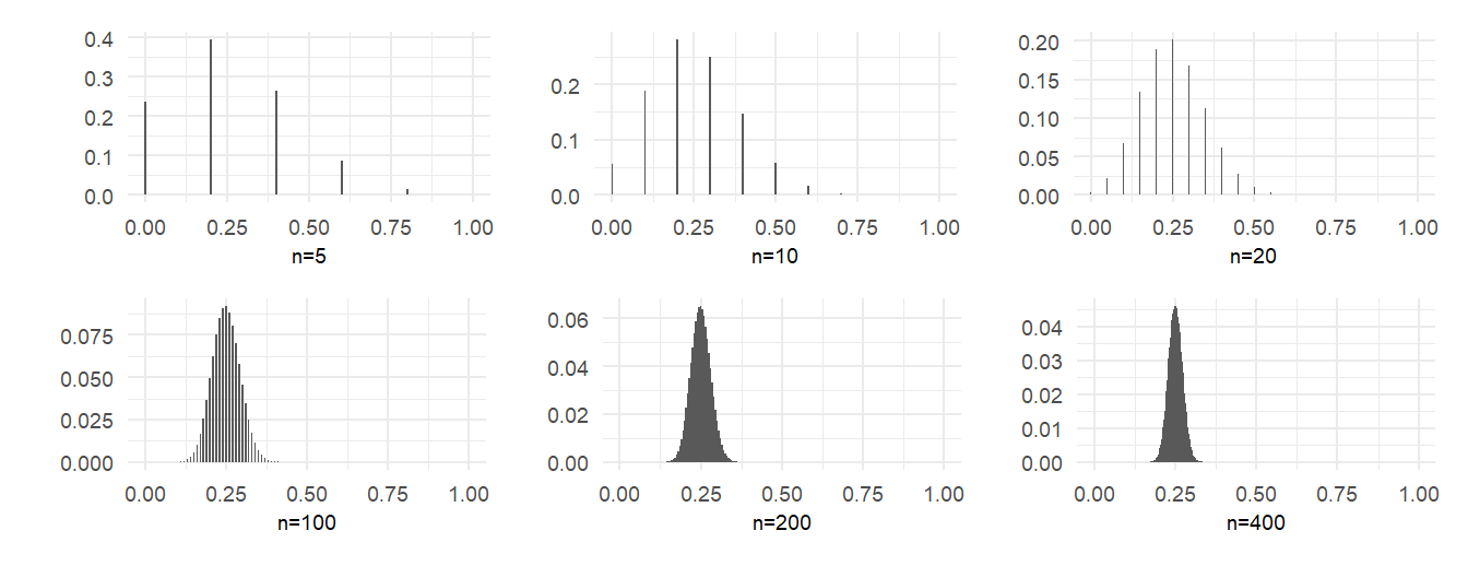
In Example 2.9 we derived the distribution of the sample mean in the coin toss example, and calculated this distribution for a fair coin with sample size 20. We repeat this exercise, this time for a coin with \(p=0.25\), for sample sizes of 5, 10, 20, 100, 200 and 400. We present the probability distribution functions graphically in Fig. 2.10. The convergence in probability of the sample mean to the true value of \(p\) can be seen in these graphs.
2.9.2 Asymptotic Normality
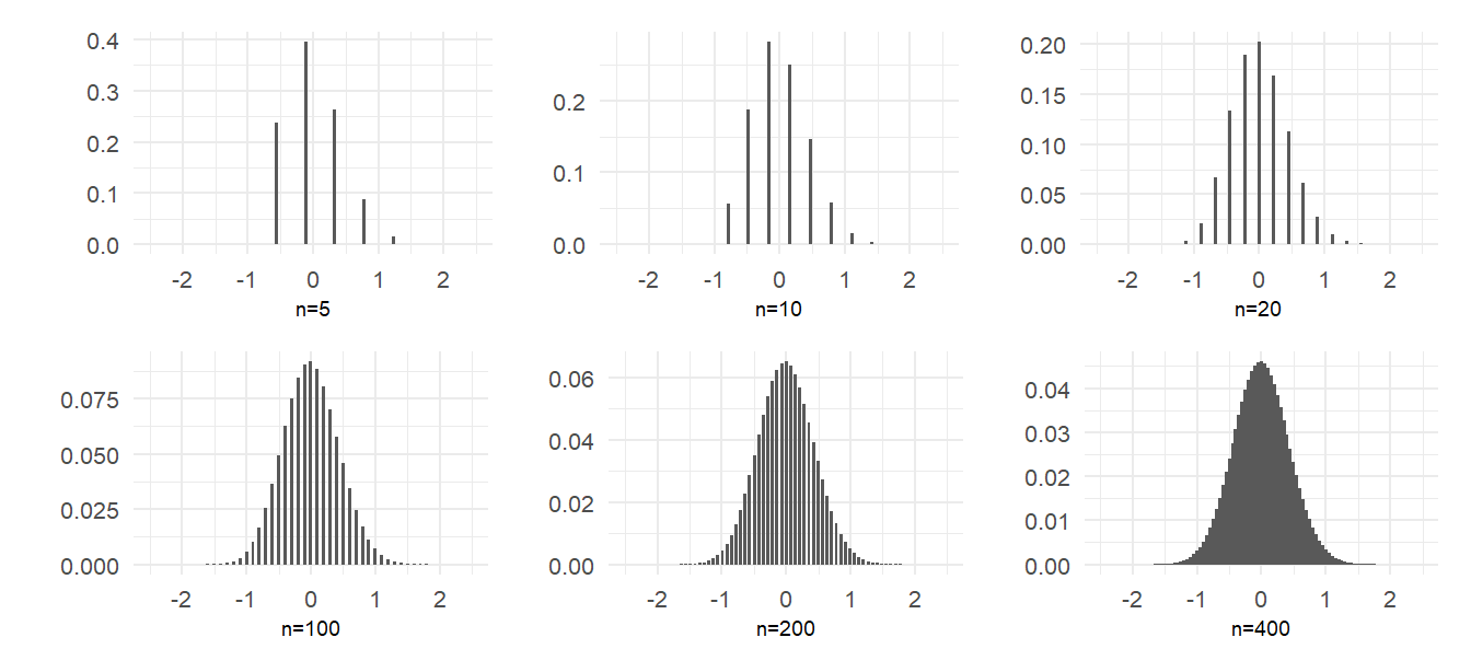
The distribution of the sample mean in the example above, with \(p=0.25\), is unsurprisingly skewed in small samples because of the low probability of heads relative to tails. However, the shape of the distribution appears to quickly becomes quite symmetric as sample size grows, and appears to converge to a familiar bell-shaped distribution. Of course, in the limit the distribution collapses to a degenerate one with all of the probability at \(p=0.25\). This is because the variance of the sample mean, \(\mathit{Var}(\hat{p})=p(1-p)/n\) goes to zero as \(n \rightarrow \infty\). Suppose, however, that we scale the sample mean (after subtracting \(p\)) by \(\sqrt{n}\), i.e., suppose we look at the distribution of \[ \sqrt{n}(\hat{p}-p). \tag{2.23}\] This random variable now has mean 0 and a non-collapsing variance \(np(1-p)/n=p(1-p)\). We can then talk about the shape of (2.23) as \(n \rightarrow \infty\) without the distribution collapsing to a single point. The plots in Fig. 2.11 show the same distributions as in Fig. 2.10, but after centering and scaling as in (2.23). The distributions appear to take the shape of a normal distribution as sample size increases.
2.9.3 The Central Limit Theorem
The convergence of the cdf of the (centered and scaled) sample mean in the coin toss example to a normal cdf is an instance of the Central Limit Theorem (CLT), a key result in probability theory. As with the law of large numbers, there are many CLTs, each listing out a set of conditions under which convergence to normality is guaranteed. We state one such CLT:
Theorem 2.2 (Lindeberg-Levy CLT) If \(\{X_i\}_{i=1}^n\) are i.i.d. with \(E(X_i) = \mu < \infty\) and \(\mathit{Var}(X_i) = \sigma^2 < \infty\) for all \(i\), then \[ \sqrt{n}(\overline{X}_n - \mu) \;\overset{d}{\rightarrow} \;\mathrm{Normal}(0,\sigma^2) \] where \(\overset{d}{\rightarrow}\) means convergence in distribution.3
Our plots of the distribution of \(\sqrt{n}(\hat{p}_n - p)\) in the coin toss example suggests convergence in distribution to \(\mathrm{Normal}(0,p(1-p))\). The sample \(\{X_i\}\) in the coin toss example does meet the requirements of the Lindeberg-Levy CLT, so in fact \(\sqrt{n}(\hat{p}_n - p) \overset{d}{\rightarrow} \mathrm{Normal}(0,p(1-p))\)
Sometimes we want to indicate that a sequence of random variables \(Y_n\) converges in distribution to the cdf of some random variable \(Y\). To so do, we write \(Y_n \overset{d}{\rightarrow} Y\).
Proposition 2.2 (Properties of convergence in distribution)
- If \(g(.)\) is a continuous function and \(Y_n \overset{d}{\rightarrow} Y\), then \(g(Y_n) \overset{d}{\rightarrow} g(Y)\).
- If \(Y_n \overset{p}{\rightarrow} Y\), then \(Y_n \overset{d}{\rightarrow} Y\).
- If \(a_n \overset{p}{\rightarrow} a\) and \(Y_n \overset{d}{\rightarrow} Y\), then \(a_n Y_n \overset{d}{\rightarrow} aY\).
Example 2.14 If \(Y_n \overset{d}{\rightarrow} Y \sim \text{Normal}(0,1)\), then \(Y_n^2 \overset{d}{\rightarrow} Y^2 \sim \chi^2(1)\), since the square of a standard normal is \(\chi^2(1)\).
Example 2.15 If \(\sqrt{n}(\overline{X}_n - \mu) \overset{d}{\rightarrow} \mathrm{Normal}(0,\sigma^2)\) and \(s_n^2\) is any consistent estimator of \(\sigma^2\), then \(1/s_n = (1/s_n^2)^{1/2}\) converges in probability to \(1/\sigma\), and therefore \[ t = \frac{\sqrt{n}(\overline{X}_n - \mu)}{s_n} = \frac{\overline{X}_n - \mu}{\sqrt{s_n^2/n}}\overset{d}{\longrightarrow} \text{Normal}(0,1). \tag{2.24}\]
If \(\sqrt{n}(\overline{X}_n - \mu) \overset{d}{\rightarrow} \mathrm{Normal}(0,\sigma^2)\), we would be justified, in large enough samples, to say that the distribution of \(\sqrt{n}(\overline{X}_n - \mu)\) is approximately \(\mathrm{Normal}(0,\sigma^2)\), or that \(\overline{X}_n\) is approximately \(\text{Normal}(\mu,\sigma^2/n)\). This last statement is sometimes written \(\overline{X}_n\overset{a}{\sim}\text{Normal}(\mu,\sigma^2/n)\), where the “\(a\)” stands for “approximately” (some take “\(a\)” to stand for “asymptotically”).
Result (2.24) is useful for hypotheses testing when one is unable or unwilling to make an assumption regarding the distribution of the population. Suppose \(\{X_i\}_{i=1}^n\) is an i.i.d. sample with \(E(X_i)=\mu\) and \(\mathit{Var}(X_i)=\sigma^2\). The sample mean \(\overline{X}_n\) is a consistent estimator for \(\mu\) and \(\widehat{\sigma^2}=\frac{1}{n-1}\sum_{i=1}^n (X_i-\overline{X}_n)^2\) is a consistent estimator for \(\sigma^2\). To test the null hypothesis \(H_0:\mu=\mu_0\), we need to compute the distribution of the sample mean, but you cannot do this unless you know the distribution of each \(X_i\). Result (2.24), however, tells us that if our sample size is large enough, then under the null hypothesis, \[ t = \frac{\overline{X}_n - \mu_0}{\sqrt{\widehat{\sigma^2}/n}} \overset{a}{\sim} \mathrm{Normal}(0,1). \tag{2.25}\] It suggests that we use the decision rule “reject the null if \(|t|>c_\alpha\)” where \(c_\alpha\) is that value such that \(\mathrm{Pr}(|t|>c_\alpha)=\alpha\), where \(\alpha\) is the chosen “level of significance” of the test, i.e., the probability of rejecting the null when it is true, and where the value \(c_\alpha\) is found from the standard normal distribution. For 0.01, 0.05, 0.10 levels of significance, the appropriate values of \(c_\alpha\) are approximately
round(qnorm(c(0.995, 0.975, 0.95)),3)[1] 2.576 1.960 1.645respectively. The 0.05 level of significance test, in particular, says to reject \(H_0:\mu=\mu_0\) if the absolute distance from the sample mean to the hypothesized value \(\mu_0\) is more than \(1.96\) (or approximately \(2\)) standard errors.
A test based on the statistic in (2.25) and rejection values (or ‘critical values’) based on the \(\mathrm{Normal}(0,1)\) distribution, would be an approximate test in the sense that the true significance level may not be exactly \(\alpha\), as intended. Nonetheless, it is a way forward in a situation where an exact test is unavailable, such as in the case of Example 2.10.
2.9.4 Working with Log-Transformed Variables
Returning to the average hourly earnings example, suppose we had computed the sample mean of \(\ln earn_i\) instead of the sample mean of \(earn_i\). Then, in an effort to obtain an estimate of the population mean of \(earn\), we take exponents of the sample mean of \(\ln earn_i\). For the data in earn2019.csv, we have
X = dat1$earn
Xbar = mean(X)
lnX = log(dat1$earn)
lnXbar = mean(lnX)
cat("sample mean of earn:", round(Xbar,2), "\n")
cat("sample mean of log earn:", round(lnXbar,2), "\n")
cat("exponent of sample mean of log earn:", round(exp(lnXbar),2), "\n")
sample mean of earn: 29.23
sample mean of log earn: 3.15
exponent of sample mean of log earn: 23.36 What are we getting? To make arguments simpler, we consider consistency instead of unbiasedness, and assume that \(earn \sim \text{Log-normal}(\mu, \sigma^2)\). Then we have \(E(\ln earn) = \mu\), and from the properties of the log-normal distribution, we have \[ E(earn) = \exp{\mu}\exp(\sigma^2/2) > \exp \mu = \mathit{Median}(earn) \] where the inequality arises because \(\exp(\sigma^2/2) > 1\). We know the sample mean of \(\ln earn_i\) is consistent for \(\mu\), i.e., \[ \frac{1}{n}\sum_{i=1}^n \ln earn_i \overset{p}\longrightarrow \mu\,, \] therefore the exponent of the sample mean of \(\ln earn_i\) is consistent for the the population median of \(earn\): \[ \exp\left( \frac{1}{n}\sum_{i=1}^n \ln earn_i \right) \overset{p}\longrightarrow \exp \mu\,. \] However, the exponent of the sample mean of \(\ln earn_i\) consistently underestimates the population mean of \(earn\).
If we want to get an estimate of \(E(earn)\) from the sample mean of \(\ln earn_i\), we have to apply a correction. Since \(\widehat{\sigma^2} \overset{p}\longrightarrow \sigma^2\), a consistent estimator for \(E(earn)\) is \[ \widehat{E(earn)} = \exp \widehat{\mu} \exp \widehat{\sigma^2}\,. \] For our data, we have
s2hat=var(lnX)
cat("exponent of sample mean of log earn, with correction :", round(exp(lnXbar)*exp(s2hat/2),2))
exponent of sample mean of log earn, with correction : 28.91which is quite close to the sample mean of \(earn\). One might argue, nonetheless, that as the distribution of \(earn\) is so skewed, the median might be a better measure of location than the mean.
2.10 Chapter 2 Exercises
Exercise 2.1 Let \(\{X_i\}_{i=1}^n\) be an iid sample from a Bernoulli distribution with parameter \(p\), i.e., \[ E(X_i) = p \;\text{ and } \; \mathit{Var}(X_i) = p(1-p)\;\text{ for all }\;i=1,\dots, n. \] An unbiased estimator for \(p\) is the sample mean \(\widehat{p} = \frac{1}{n}\sum_{i=1}^n X_i = \overline{X}\). Since \(\mathit{Var}(\widehat{p}) = p(1-p)/n\), consider estimating \(\mathit{Var}(\widehat{p})\) using \[ \widehat{\mathit{Var}}(\widehat{p}) = \frac{\widehat{p}(1-\widehat{p})}{n}\,. \] Show that this is equivalent to using \[ \widetilde{\mathit{Var}}(\hat{p}) = \frac{\widetilde{\sigma^2}}{n} \] where \[ \widetilde{\sigma^2} = \frac{1}{n}\sum_{i=1}^n(X_i - \overline{X})^2\,. \]
Exercise 2.2 Given a sample \(\{X_i\}_{i=1}^n\), consider a weighted average \[ \widetilde{X} = \sum_{i=1}^n w_i X_i = w_1 X_1 + w_2 X_2 + \dots w_n X_n\, \] as an estimator for the population mean. The sample mean \(\overline{X}\) is a special case of \(\widetilde{X}\) with \(w_i = 1/n\) for all \(i=1, \dots, n\). Show that \(\widetilde{X}\) is an unbiased estimator for the population mean as long as \(\sum_{i=1}^n w_i = 1\). Assuming that \(\sum_{i=1}^n w_i = 1\), show that \[ \mathit{Var}(\widetilde{X}) \geq \mathit{Var}(\overline{X})\,. \]
Exercise 2.3 A measure of the quality of an estimator \(\widehat{\theta}\) for a parameter \(\theta\) is the mean squared estimation error \[ MSE(\widehat{\theta}) = E((\theta - \widehat{\theta})^2)\,. \] Show that \[ MSE(\widehat{\theta}) = Bias(\widehat{\theta})^2 + \mathit{Var}(\widehat{\theta}) \] where \(Bias(\widehat{\theta}) = E(\widehat{\theta}) - \theta\).
Exercise 2.4 It can be shown that if \(Y_i\), \(i=1,2,...,n\) are iid draws from a normal distribution with mean \(\mu\) and variance \(\sigma^2\), then the variance of the unbiased variance estimator \[ \widehat{\sigma^2} = \frac{1}{n-1}\sum_{i=1}^n (Y_i - \overline{Y})^2 \] is \[ \mathit{Var}(\widehat{\sigma^2})=\dfrac{2\sigma^4}{n-1}\,. \] For this question, you may take the above fact as given. Because \(\widehat{\sigma^2}\) is unbiased, its MSE also has the same expression.
(a) Show that the biased estimator \(\widetilde{\sigma^2} = \dfrac{1}{n}\sum\limits_{i=1}^n (Y_i - \overline{Y})^2\) has a smaller variance than \(\widehat{\sigma^2}\).
(b) Show that \(MSE(\widetilde{\sigma^2}) = \dfrac{2n-1}{n^2}\sigma^4\).
(c) Show that \(MSE(\widetilde{\sigma^2}) < MSE(\widehat{\sigma^2})\).
This is an example where a biased estimator might be prefered to an unbiased one. Here the MSE of the unbiased estimator is lowered by reducing variance at the expense of a little bit of bias.
Exercise 2.5 The quantile function qnorm(p, mean, sd), when evaluated at probability \(p\), returns the value of \(c\) for which \(\Pr(X\leq c) = p\), when \(X \sim \mathrm{Normal(mean, sd^2)}\). The default values of mean and sd are 0 and 1 respectively. For example:
qnorm(0.5) # c such that Pr(X<=c)=0.5 when X~N(0,1)[1] 0The corresponding functions for the student-t, chi-sq, and F distributions are qt(p, df), qchisq(p,df), and qf(p,df1, df2) respectively.
(a) For \(p = 0.01, 0.05, 0.10\), plot the lines \(c\) and \(-c\) against \(v\) such that
\(\Pr(\lvert X \rvert > c) = p\) when \(X\sim \mathrm{t}(v)\) for \(v=10, 20, \dots, 200\).
\(\Pr(\lvert X \rvert > c) = p\) when \(X\sim \text{Normal}(0,1)\). (This will be two constant lines.)
The code to do (a) is given below.
v <- seq(10, 200, 10)
c1 <- qt(0.995, v); c2 <- qt(0.975, v); c3 <- qt(0.95, v)
n1 <- qnorm(0.995); n2 <- qnorm(0.975); n3 <- qnorm(0.95)
plt_df <- data.frame(c1=c1, n1=n1, c2=c2, n2=n2, c3=c3, n3=n3, v=v)
p1 <- ggplot(data=plt_df) +
  geom_line(aes(y= c1, x=v), linetype='dashed', color='cadetblue', linewidth=1) +
  geom_line(aes(y=-c1, x=v), linetype='dashed', color='cadetblue', linewidth=1) +
  geom_line(aes(y= n1, x=v), linetype='solid', color ='cadetblue', linewidth=1) +
  geom_line(aes(y=-n1, x=v), linetype='solid', color ='cadetblue', linewidth=1) +
  geom_line(aes(y= c2, x=v), linetype='dashed', color='chocolate', linewidth=1) +
  geom_line(aes(y=-c2, x=v), linetype='dashed', color='chocolate', linewidth=1) +
  geom_line(aes(y= n2, x=v), linetype='solid', color ='chocolate', linewidth=1) +
  geom_line(aes(y=-n2, x=v), linetype='solid', color ='chocolate', linewidth=1) +
  geom_line(aes(y= c3, x=v), linetype='dashed', color='darkorchid', linewidth=1) +
  geom_line(aes(y=-c3, x=v), linetype='dashed', color='darkorchid', linewidth=1) +
  geom_line(aes(y= n3, x=v), linetype='solid', color ='darkorchid', linewidth=1) +
  geom_line(aes(y=-n3, x=v), linetype='solid', color ='darkorchid', linewidth=1) +
  theme_bw() + ylim(-3.5,3.5) + xlim(1, 200)
p1
(b) For \(p = 0.01, 0.05, 0.10\), plot the lines \(c\) against \(v\) such that \(\Pr(X > c) = p\) when \(X\sim \chi^2(v)\) for \(v=10, 20, \dots, 200\).
(c) For \(p = 0.01, 0.05, 0.10\), plot the lines \(c\) against \(v_2\) such that \(\Pr(X > c) = p\) when \(X\sim F(v_1, v_2)\) for \(v_2=10, 20, \dots, 200\). Do this for \(v_1 = 2, 3, 4, 5\), one figure per value of \(v_1\).
2.11 Appendix: The Summation Notation
The uppercase sigma “\(\Sigma\)” is used to denote summation. For a set of numbers \(\{x_{1}, x_{2}, \dots, x_{n}\}\), define \[ \sum_{i=1}^{n} x_{i} = x_{1} + x_{2} + \dots + x_{n}\,. \]
Example 2.16 The sample average (also sample mean, arithmetic mean) of a set of numbers \(\{x_{1}, x_{2}, \dots, x_{n}\}\) is \[ \overline{x}= \frac{1}{n}\sum_{i=1}^{n} x_{i}\,. \]
Example 2.17 Write the sum \(4+8+12+16+20+24\) in summation notation. Ans: \(\sum_{i=1}^{6} 4i\).
Example 2.18 In economics and finance, the present value of a future amount of money is the amount today that, if invested at a certain rate, returns that future sum. Suppose the following payments are to be made: \(a_1\) at the end of the first period, \(a_2\) at the end of the second period, and so on, for \(n\) periods. At a fixed interest rate of \(r\) per period, the present value of the payments is \[ \frac{a_{1}}{1+r} + \frac{a_{2}}{(1+r)^{2}} + \dots + \frac{a_{n}}{(1+r)^{n}} = \sum_{i=1}^{n} \frac{a_{i}}{(1+r)^{i}}\,. \]
Example 2.19 \(\sum_{i=1}^{n} c = nc\).
Expressions using the summation notation are not unique.
Example 2.20 Write \(1 - \frac{1}{3} + \frac{1}{5} - \frac{1}{7} + \frac{1}{9} - \frac{1}{11}\) in summation notation. \[ \begin{aligned} \text{Ans: } &\sum_{i=1}^{6} (-1)^{i-1}\frac{1}{2i-1}. \\[1ex] \text{Alternative Ans: } &\sum_{i=0}^{5} (-1)^{i} \frac{1}{2i+1}\,. \end{aligned} \]
2.11.0.1 Rules for summation notation
The summation notation greatly simplifies notation but this is only helpful if you know how to manipulate expressions written using it. There are only two rules to learn: \[ \begin{aligned} \text{i.} \qquad&\sum_{i=1}^{n} (a_{i} + b_{i}) = \sum_{i=1}^{n} a_{i} + \sum_{i=1}^{n} b_{i} \\ \text{ii.} \qquad&\sum_{i=1}^{n} (ca_{i}) = c\sum_{i=1}^{n} a_{i}\;\;\text{where} \;\;c\;\; \text{is some constant.} \end{aligned} \]
Example 2.21 Given any set of numbers \(\{x_{1}, x_{2}, \dots, x_{n}\}\), we have \[ \sum_{i=1}^{n} (x_{i} - \overline{x}) = 0 \,. \] That is, the sum of deviations of any set of numbers from its sample average is always zero.
Proof: \(\sum_{i=1}^{n} (x_i - \overline{x})=\sum_{i=1}^{n} x_{i} -\sum_{i=1}^{n} \overline{x} = n \overline{x} - n \overline{x} = 0\).
Example 2.22 Given \(n\) pairs of numbers \((x_{i},y_{i})\), \(i=1,2,...,n\), we have \[ \sum_{i=1}^n (x_{i}-\overline{x})(y_{i}-\overline{y}) = \sum_{i=1}^n (x_{i}-\overline{x})y_{i} = \sum_{i=1}^n (y_{i}-\overline{y})x_{i}\,. \tag{2.26}\]
Proof: For the first equality in (2.26), we have \[ \begin{aligned} \sum_{i=1}^{n} (x_{i}-\overline{x})(y_{i}-\overline{y}) \; &=\; \sum_{i=1}^{n} (x_{i}-\overline{x})y_{i}-\sum_{i=1}^{n} (x_{i}-\overline{x})\overline{y} \\ &=\; \sum_{i=1}^{n} (x_{i}-\overline{x})y_{i}-\overline{y}\underbrace{\sum_{i=1}^{n} (x_{i}-\overline{x})}_{=\,0} \;=\; \sum_{i=1}^{n} (x_{i}-\overline{x})y_{i}. \end{aligned} \] The second equality in (2.26) can be shown in similar fashion.
How to actually do this is the subject of the field called “survey sampling”.↩︎
Note that the mean and variance need not actually be separate parameters. In the case of the normal, they are indeed separate, but in the Poisson, both the mean and variance are equal to \(\lambda\). In the binomial we have \(E(X) = p\) and \(\mathit{Var}(X) = p(1-p)\). In the log-normal, there are two parameters typically called \(\mu\) and \(\sigma^2\) but these do not represent the mean and variance of \(X\). In what follows, I will use \(\mu\) and \(\sigma^2\) to represent the mean \(E(X)\) and variance \(\mathit{Var}(X)\) of \(X\), no matter what the actual distribution of \(X\) is.↩︎
Technically, this means that the cumulative distribution function (cdf) of the random variable on the left converges pointwise to the cdf of the distribution indicated on the right.↩︎