library(tidyverse) # For data handling and visualization7 Topics in OLS Estimation of the Linear Regression Model
This chapter serves two purposes: One, it is a summary of the theory we have covered to this point. Second, we discuss can some of the things that can go wrong in least squares estimation of the linear regression model. As to what to do when such-and-such problem arises, this will only be partly answered in this chapter. Many of the issues discussed here require more advanced theory presented in the next few chapter.
The R code in this chapter uses the following package (and one call to the sandwich package).
7.1 Recap
The linear regression model estimates population conditional expectation which is assumed to be linear-in-parameters: \[ E(Y \mid X_1, \dots, X_{K-1}) = \beta_0 + \beta_1 X_1 + \dots + \beta_{K-1} X_{K-1}. \] The regressors \(X_1,\dots,X_{K-1}\) may be distinct variables, but some may be transformations of or interactions between other regressors, e.g., we can have \[ E(\ln earn \mid age, educ) = \beta_0 + \beta_1 age + \beta_2 age^2 + \beta_3 educ + \beta_4 male + \beta_5 male \cdot educ. \] We can write the regression model as \[ Y = E(Y \mid X_1, \dots, X_{K-1}) + \epsilon = \beta_0 + \beta_1 X_1 + \dots + \beta_{K-1} X_{K-1} + \epsilon\,. \] As long as the conditional expectation is correctly specified, we have \[ E(\epsilon \mid X_1, \dots, X_{K-1}) = 0\,. \] Follow on implications are that \(E(\epsilon) = 0\), and \(E(\epsilon X_k) = 0\) for \(k=0, \dots, K-1\). Another way of describing the latter set of conditions is that the noise variable \(\epsilon\) is uncorrelated with each of the regressors \(X_1, \dots, X_{K-1}\).
The classical linear regression model adds the assumption \(\mathit{Var}(\epsilon \mid X_1, \dots, X_{K-1}) = \sigma^2\). Since \(\epsilon\) has zero conditional mean, this “homoskedasticity” assumption can be (and often is) written as \(E(\epsilon^2 \mid X_1, \dots, X_{K-1}) = \sigma^2\).
If you have a representative iid sample \(\{Y_i, X_{i1}, \dots, X_{i,K-1}\}_{i=1}^n\) from the population (we assume cross-sectional samples for the moment), we can write \[ Y_i = \beta_0 + \beta_1 X_{i1} + \dots + \beta_{K-1} X_{i,K-1} + \epsilon_i\,,i = 1, \dots, n\,, \] where \[ \begin{aligned} E(\epsilon_i &\mid X_{11}, \dots, X_{n1}; \dots; X_{1, K-1}, \dots, X_{n,K-1}) = 0 \\ E(\epsilon_i^2 &\mid X_{11}, \dots, X_{n1}; \dots; X_{1, K-1}, \dots, X_{n,K-1}) = \sigma^2 \\ E(\epsilon_i \epsilon_j &\mid X_{11}, \dots, X_{n1}; \dots; X_{1, K-1}, \dots, X_{n,K-1}) = 0 \end{aligned} \] for all \(i,j = 1, \dots, n\), \(i \neq j\). All this can be written in matrix form as \[ y = X\beta + \varepsilon\,,\,E(\varepsilon \mid X) = 0\,,\,\,E(\varepsilon \varepsilon^\mathrm{T} \mid X) = \sigma^2 I_n\,. \] The OLS estimator for \(\beta\) is \[ \widehat\beta^{ols} = (X^\mathrm{T}X)^{-1}X^\mathrm{T}y\,. \] This requires \(X^\mathrm{T}X\) to be invertible, which will be the case if the columns of \(X\) are linearly independent, meaning that \[ Xc = 0_n \Longleftrightarrow c = 0_K\,. \] If there is a \(c \neq 0_K\) such that \(Xc = 0_n\), than you have a “perfect collinearity” situation, and OLS is infeasible. In practice, your OLS estimates can be unreliable or infeasible if the columns of \(X\) are “nearly perfectly collinear”, a situation we call “multicollinearity”. OLS might be infeasible because the computations (particularly the inverting of \(X^\mathrm{T}X\)) become numerically unstable. Even where OLS is feasible, you will generally get large standard errors where there is strong multicollinearity.
Having obtained OLS estimates, the OLS fitted values can be calculated as \(\widehat{y}_{ols} = X\widehat{\beta}^{ols}\) and the OLS residuals can be calculated as \(\widehat{\varepsilon}_{ols} = y - \widehat{y}_{ols}\).
If \(E(\varepsilon \mid X) = 0\), the OLS estimator is unbiased. If the homoskedasticity assumption holds, then \(\mathit{Var}(\widehat\beta_{ols} \mid X) = \sigma^2(X^\mathrm{T}X)^{-1}\). The noise variance \(\sigma^2\) can be estimated using \[ \widehat{\sigma^2} = \frac{\widehat{\varepsilon}_{ols}^\mathrm{T}\widehat{\varepsilon}_{ols}}{n-K}\,. \] An estimator of the variance-covariance matrix of \(\widehat{\beta}^{ols}\) is then \[ \widehat{\mathit{Var}}(\widehat{\beta}^{ols} \mid X) = \widehat{\sigma^2}(X^\mathrm{T}X)^{-1}\,. \] If errors are homoskedastic, than the OLS estimators of the linear regression model turns out to be “Best Linear Unbiased”. That is, given any other linear unbiased estimator \(\widetilde{\beta}\) of the linear regression model, we have \[ \mathit{Var}(c^\mathrm{T}\widehat{\beta}^{ols} \mid X) \leq \mathit{Var}(c^\mathrm{T}\widetilde{\beta} \mid X) \] for any \(K \times 1\) vector \(c \neq 0_K\). For goodness-of-fit, the \(R^2\) statistic \[ R^2 = 1 - \frac{\widehat{\varepsilon}_{ols}^\mathrm{T}\widehat{\varepsilon}_{ols}}{y^\mathrm{T}M_0y} = 1 - \frac{RSS}{TSS} \] measures the proportion of variation in \(Y_i\) is accounted for by the explanatory variables. It has the feature that \(0 \leq R^2 \leq 1\), as long as an intercept is included and estimation was done by ordinary least squares. The \(R^2\) never decreases (and usually increases) as more regressors are included in the regression. To counter this, the adjusted-\(R^2\) \[ \text{adj.-}R^2 = 1 - \frac{RSS/{n-K}}{TSS/{n-1}}\,. \] is sometimes reported.
For testing the single hypothesis \(H_0: r^\mathrm{T}\beta = r_0 \quad \text{vs} \quad r^\mathrm{T}\beta \neq r_0\), where \(r\) is \(K \times 1\) and \(r_0\) is a scalar, we can use the \(t\)-test \[ t = \frac{r^\mathrm{T}\hat{\beta} - r_0}{\sqrt{ r^\mathrm{T}\widehat{\mathit{Var}}(\hat{\beta}^{ols} \mid X)r}}\,. \] For multiple hypotheses \(H_0: \mathcal{R}\beta = r_0 \quad \text{vs} \quad H_A: \mathcal{R}\beta \neq r_0\), where \(\mathcal{R}\) is a \((J \times K)\) matrix and \(r_0\) is a \((J \times 1)\) vector, you can use the \(F\)-test \[ \begin{aligned} F &= \frac{(\hat{\varepsilon}_{rls}^\mathrm{T}\hat{\varepsilon}_{rls} - \hat{\varepsilon}_{ols}^\mathrm{T}\hat{\varepsilon}_{ols}) / J} {\hat{\varepsilon}^\mathrm{T}\hat{\varepsilon} / (n-K)} \\[1ex] &=\frac{(R_{ur}^2 - R_r^2)/J}{(1-R_{ur}^2)/(n-K)} \\[2ex] &= (\mathcal{R}\hat{\beta}-r_0)^\mathrm{T} (\mathcal{R}\,\widehat{\mathit{Var}}(\hat{\beta}^{ols} \mid X)\,\mathcal{R}^\mathrm{T})^{-1} (\mathcal{R}\hat{\beta}-r_0)/J \end{aligned} \] where \(\hat{\varepsilon}_{rls}\) are the restricted least squares estimator of \(\beta\), \(R_{r}^2\) is the \(R^2\) of this restricted regression, and \(R_{ur}^2\) is the \(R^2\) of the unrestricted regression. If the noise terms \(\epsilon_i\) are normally distributed, then \[ t \sim \text{t}(n-K) \;\;\text{ and }\;\; F \sim \text{F}(J, n-K)\,. \] Otherwise, we can usually rely on large-sample approximate tests \[ t \overset{a}{\sim} \text{Normal}(0,1) \;\;\text{ and }\;\; JF \overset{a}{\sim} \chi^2(J)\,. \]
Over the next few sections, we mention some of the things that can go wrong in a regression analysis, some of which we have already mentioned previously. Where feasible, we will say something about how we might detect that there is a problem in the first place, and how to fix it. In other cases (particularly the later examples in this chapter), the “fixes” will be discussed in later chapters. We begin with two fairly innocuous assumptions, normality of the noise term and homoskedasticity.
7.2 Normality of Noise Term
Non-normality of errors does not affect unbiasedness or consistency of the OLS estimator. Most of the theory of OLS stands without this assumption. Its primary function is to provide the finite sample distribution for the \(t\)- and \(F\)-statistics. One way to test for normality is to use the fact that a normal random variate has skewness coefficient is zero (because it is symmetric), and its kurtosis coefficient is three: if \(X \sim \text{Normal}(\mu, \sigma^2)\), then \[ S = E((X-\mu)^3)/\sigma^3 = 0 \;\;\text{ and }\;\; Kur = E((X-\mu)^4)/\sigma^4 = 3\,. \] The kurtosis coefficient, being the expectation of a fourth moment, emphasizes larger deviations from mean over small deviations from mean (deviations from mean less than one become very small when raised to the fourth power). A kurtosis coefficient greater than 3 suggests higher probability of large deviations from mean, relative to a comparable normally distributed random variable. The skewness and kurtosis coefficients can be estimated using \[ \widehat{S} = \frac{\frac{1}{n}\sum_{i=1}^n(X_i-\overline{X})^3} {\left[\frac{1}{n}\sum_{i=1}^n(X_i-\overline{X})^2\right]^{3/2}} \,\,\text{ and }\;\; \widehat{Kur} = \frac{\frac{1}{n}\sum_{i=1}^n(X_i-\overline{X})^4} {\left[\frac{1}{n}\sum_{i=1}^n(X_i-\overline{X})^2\right]^{2}} \,. \] The Jarque-Bera statistic applies this idea to regression residuals, using the statistic \[ JB = \frac{n-K}{6}\left(\widehat{S}^2 + \frac{1}{4}(\widehat{Kur} - 3)^2\right) \] which is approximately \(\chi^2(2)\) in large samples under the null. Some implementations ignore the degree-of-freedom correction and use \(n\) in the numerator instead of \(n-K\).
We test for normality of the residuals in the regression \[ \ln earn_i = \beta_0 + \beta_1 \ln wexp_i + \beta_2 \ln tenure_i + \epsilon_i \]
Skew <- function(x){
  return(mean((x-mean(x))^3)/(mean((x-mean(x))^2)^(3/2)))
}
Kurt <- function(x){
  return(mean((x-mean(x))^4)/(mean((x-mean(x))^2)^2))
}
JB <- function(mdl){
  # requires lm object, returns JB Stat, p-val, Skewness and Kurtosis Coef.
  N <- nobs(mdl)
  K <- summary(mdl)$df[1]
  ehat <- residuals(mdl)
  JBSkew <- Skew(ehat)
  JBKurt <- Kurt(ehat)
  JBstat <- ((N-K)/6*(JBSkew^2 + (1/4)*(JBKurt-3)^2))
  JBpval <- 1-pchisq(JBstat,2)
  return(list("JBstat"=JBstat, "JBpval"=JBpval, "Skewness"=JBSkew, "Kurtosis"=JBKurt))
}

df_earn <-read_csv("data\\earnings2019.csv",show_col_types=FALSE)
mdl <- lm(log(earn)~log(wexp)+log(tenure), data=df_earn)
JBtest <- JB(mdl)
fmt <- function(x){format(round(x,4),nsmall=4)}
cat("JB:", fmt(JBtest$JBstat), "  p-val:", fmt(JBtest$JBpval),
    "  Skewness:", fmt(JBtest$Skewness), "  Kurtosis:", fmt(JBtest$Kurtosis),"\n")
JB: 338.6182 p-val: 0.0000 Skewness: 0.0816 Kurtosis: 4.2718 The null of normality is rejected. The distribution is quite symmetric, but there is ‘excess kurtosis’ (kurtosis in excess of 3). A histogram of the OLS residuals is shown below.
hist(residuals(mdl), 20)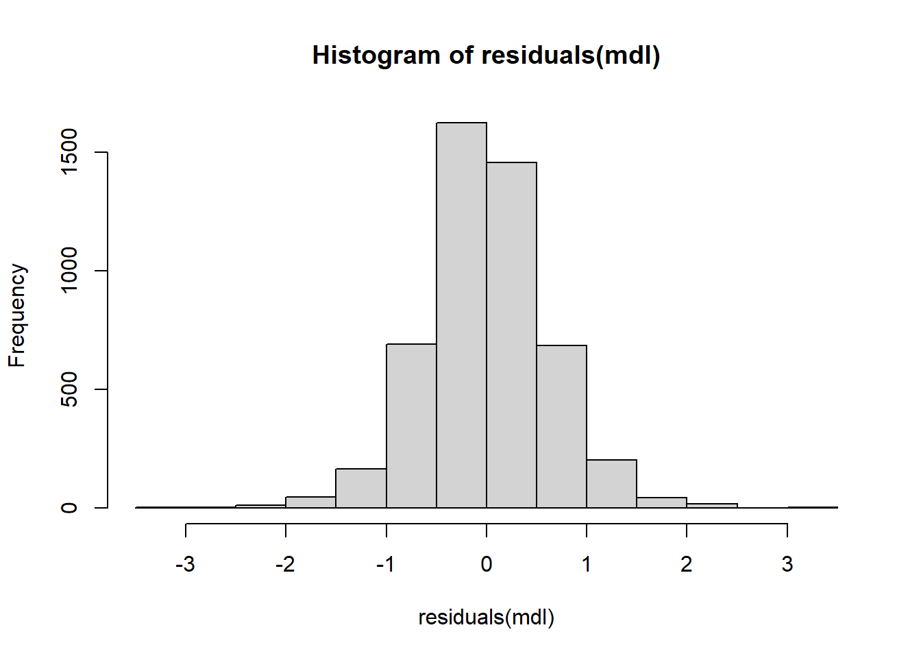
The problem with highly skewed and very fat-tailed noise distributions is that the CLT may converge slowly, so that the asymptotic tests may be poor approximations unless sample size is sufficiently large. Here we do not have a skewness problem, but the estimated kurtosis is above four, which is probably large enough that we would want a reasonably large sample size. We have almost 5000 observations which should be more than enough. Sometimes the \(Y\) variable is transformed to make the noise term “more normal”. In fact, in our example our log transformation of \(earn\) contributes substantially to the normality of the noise term.
7.3 Heteroskedasticity
We know that heteroskedasticity of the noise terms does not affect the unbiasedness or consistency of OLS estimators of the linear regression model. As explained in previous chapters, the only concern regarding heteroskedasticity when using OLS is to calculate the standard errors properly. In particular, we ought to use \[ \widehat{\mathit{Var}}_{HC0}(\hat\beta^{ols}) = \left(\sum_{i=1}^n X_{i*}^\mathrm{T}X_{i*}\right)^{-1} \left(\sum_{i=1}^n \hat{\epsilon}_i^2X_{i*}^\mathrm{T}X_{i*}\right) \left(\sum_{i=1}^n X_{i*}^\mathrm{T}X_{i*}\right)^{-1} \] or one of its variants, instead of the usual \(\widehat{\sigma^2}(X^\mathrm{T}X)^{-1}\). The benefit of using the heteroskedasticity-robust variance-covariance matrix is that it remains consistent for \(\mathit{Var}(\widehat\beta^{ols})\) even under homoskedasticity, so one can argue that standard errors reported by programs ought to be obtained from it by default.1 The heteroskedasticity-robust version can also be used in the expressions for the \(t\) and \(F\) statistics, replacing \(\widehat{\mathit{Var}}(\widehat\beta^{ols})\), to get heteroskedasticity-robust t and F tests.
We know, however, that OLS estimators are efficient when the noise terms are homoskedastic, and may not be so otherwise. The question, then, is whether or not we can do better than OLS in terms of getting more precise estimators when the noise terms are heteroskedastic.
We begin with a simple illustrative example where we can directly show the inefficiency of OLS under heteroskedasticity.
Example 7.1 Suppose \[ Y_i = \beta_1 X_{i1} + \epsilon_i \, , \, i=1,2,...,n\,. \tag{7.1}\] We assume all of the usual OLS assumptions continue to hold, except that \[ E(\epsilon_{i}^2 \mid X_{11}, \dots, X_{n1}) = \sigma^2X_{i1}^2 \;\;\text{ for all }\; i=1, \dots, n\,. \] The OLS estimator for \(\beta_1\) in this example is \[ \hat{\beta}_1^{ols} = \frac{\sum_{i=1}^N X_{i1}Y_i}{\sum_{i=1}^N X_{i1}^2} \tag{7.2}\] which is unbiased for \(\beta_1\) (see exercises). Under our assumptions, the variance of the OLS estimator is \[ \begin{aligned} \mathit{Var}(\hat{\beta}_1^{ols} \mid X_{11}, \dots, X_{n1}) &= \frac{\sum_{i=1}^N X_{i1}^2\mathit{Var}(\epsilon_i\mid X_{11}, \dots, X_{n1})}{\left(\sum_{i=1}^N X_{i1}^2\right)^2} \\[1.5ex] &= \frac{\sum_{i=1}^N X_{i1}^2(\sigma^2 X_{i1}^2)}{\left(\sum_{i=1}^N X_{i1}^2\right)^2} \\[1.5ex] &= \frac{\sigma^2\sum_{i=1}^N X_{i1}^4}{\left(\sum_{i=1}^N X_{i1}^2\right)^2}\,. \end{aligned} \tag{7.3}\] We will show that this estimator is inefficient, by presenting a more efficient linear unbiased estimator. First, weight each observation by \(1/X_{i1}\) and run the regression \[ \frac{Y_i}{X_{i1}} = \beta_1 + \frac{\epsilon_i}{X_{i1}} = \beta_1 + \epsilon_i^*\,. \tag{7.4}\] That is, simply regress \(Y_{i}/X_{i1}\) on a constant. The modified noise terms in this regression will continue to have zero conditional expectation \[ E(\epsilon_i/X_{i1} \mid X_{i1}, \dots, X_{n1}) = (1/X_{i1})E(\epsilon_i \mid X_{i1}, \dots, X_{n1}) = 0 \] and remain uncorrelated (exercise). Furthermore, its conditional variance is now constant: \[ \mathit{Var}(\epsilon_i/X_{i1} \mid X_{i1}, \dots, X_{n1}) = (1/X_{i1}^2)\mathit{Var}(\epsilon_i \mid X_{i1}, \dots, X_{n1}) = \sigma^2\,. \] OLS estimation applied to this modified regression model (7.4) gives the estimator \[ \hat{\beta}_1^{wls} = \frac{1}{n}\sum_{i=1}^n\frac{Y_i}{X_{i1}} \,. \tag{7.5}\] The ‘wls’ superscript stands for “weighted least squares”. It is easy to show that (7.5) is unbiased (exercise). Since (7.5) can be written as \[ \hat{\beta}_1^{wls} = \sum_{i=1}^{n} \left( \frac{1}{nX_{i1}}\right) Y_i\,, \] it is also a linear estimator. In fact, it is BLU since the regression satisfies all the necessary conditions for OLS to be BLU. The fact that \(\hat{\beta}_1^{wls}\) is BLU suggests that \(\hat{\beta}_1^{ols}\) is not. In our simple example, it is straightforward to directly demonstrate that \[ \mathit{Var}(\hat{\beta}_1^{wls} \mid X_{11}, \dots, X_{n1}) \leq \mathit{Var}(\hat{\beta}_1^{ols} \mid X_{11}, \dots, X_{n1})\,. \] Since \(\hat{\beta}_1^{wls}\) is a sample mean of \(n\) observations of a random variable with variance \(\sigma^2\), its variance is \[ \mathit{Var}(\hat{\beta}_1^{wls}\mid X_{11}, \dots, X_{n1}) = \frac{\sigma^2}{n}\,. \tag{7.6}\] It can be shown (see exercises) that \[ \frac{\sum_{i=1}^n X_{i1}^4}{\left(\sum_{i=1}^n X_{i1}^2\right)^2} \geq \frac{1}{n}\,, \tag{7.7}\] therefore \[ \mathit{Var}(\hat{\beta}_1^{wls}\mid X_{11}, \dots, X_{n1}) = \frac{\sigma^2}{n} \leq \frac{\sigma^2\sum_{i=1}^N X_{i1}^4}{\left(\sum_{i=1}^N X_{i1}^2\right)^2} = \mathit{Var}(\hat{\beta}_1^{ols}\mid X_{11}, \dots, X_{n1})\,. \] The reason OLS estimators are inefficient when there is conditional heteroskedasticity is that the observations with large noise variances are less informative about the population regression line than the ones with smaller noise variances, but OLS makes no use of this fact. Information ignored leads to inefficiency. The weighted least squares approach, on the other hand, uses this information directly by assigning less weight to noisier observations, and more weight to observations whose noise terms have lower variance.
7.3.1 Weighted Least Squares
Suppose our linear regression model is \[ Y_i = \beta_0 + \beta_1 X_{i1} + \dots + \beta_{K-1} X_{i, K-1} + \epsilon_i \,,\,i=1, \dots, n, \] with \(E(\epsilon_i \mid X) = 0\,,\,i=1, \dots, n\), \(E(\epsilon_i \epsilon_j \mid X) = 0\), \(i,j=1, \dots, n\) and \(i \neq j\), and \[ E(\epsilon_i^2 \mid X) = \sigma_i^2 = \sigma^2 \eta_i\,,\,i=1, \dots, n \] where \(\eta_i\) is a completely known function of the regressors. In other words, in \(\sigma^2 \eta_i\), the only unknown parameter is \(\sigma^2\). For instance, \[ \sigma_i^2 = \sigma^2 \lvert X_i \rvert\;\;\text{ or }\;\; \sigma_i^2 = \sigma^2 X_i^2 \;\;\text{ or } \sigma_i^2 = \sigma^2 \exp(X_i)\,. \] Put yet another way, we assume the form of conditional heteroskedasticity is completely known up to a constant factor.
The idea of weighted least squares is to weight each observation so that the weighted noise terms are no longer heteroskedastic. That is, we modify the regression equation to \[ \frac{Y_i}{\sqrt{\eta_i}} = \beta_0\frac{1}{\sqrt{\eta_i}} + \beta_1 \frac{X_{i1}}{\sqrt{\eta_i}} + \dots + \beta_{K-1}\frac{X_{i,K-1}}{\sqrt{\eta_i}} + \frac{\epsilon_i}{\sqrt{\eta_i}} \] which we can write as \[ Y_i^* = \beta_0X_{0,i}^* + \beta_1 X_{i1}^* + \dots + \beta_{K-1} X_{i,K-1}^* + \epsilon_i^*\,. \tag{7.8}\] Since \(\eta_i\) is fixed conditional on the regressors, we have \[ \begin{aligned} E({\epsilon_{i}^{*}} \mid X) &= E\left( \left( \frac{\epsilon_{i}}{\sqrt{\eta_{i}}}\right) \;\Bigg\vert\; X \right) = \frac{1}{\sqrt{\eta_{i}}} E(\epsilon_{i} \;\mid\; X ) = 0\;;\\[1ex] E({\epsilon_{i}^{*}}^2 \mid X) &= E\left( \left( \frac{\epsilon_{i}}{\sqrt{\eta_{i}}}\right)^{2} \;\Bigg\vert\; X \right) = \frac{1}{\eta_{i}} E(\epsilon_{i}^{2} \;\mid\; X ) = \frac{1}{\eta_{i}}{\sigma^2 \eta_i} = \sigma^{2}\;;\\[1ex] E({\epsilon_{i}^{*}\epsilon_{j}^{*}} \mid X) &= E\left( \left( \frac{\epsilon_{i}\epsilon_{j}}{\sqrt{\eta_{i}}\sqrt{\eta_{j}}}\right) \;\Bigg\vert\; X \right) = \frac{1}{\sqrt{\eta_{i}}\sqrt{\eta_{j}}} E(\epsilon_{i}\epsilon_{j} \;\mid\; X ) = 0\;. \end{aligned} \] OLS estimation of (7.8) will produce BLU estimators of the coefficients since all the necessary conditions for OLS to be BLU are met.
Applying OLS on the transformed regression equation (7.8) is equivalent to choosing \(\hat{\beta}_0, \hat{\beta}_1, \hat{\beta}_{K-1}\) to minimize \[ \begin{aligned} &\sum_{i=1}^n (Y_i^* - \hat\beta_0X_{i0}^* - \hat\beta_1 X_{i1}^* - \dots - \hat\beta_{K-1} X_{i,K-1}^*)^2 \\ = &\sum_{i=1}^n (Y_i/\sqrt{\eta_i} - \hat\beta_0(1/\sqrt{\eta_i}) - \hat\beta_1 X_{i1}/\sqrt{\eta_i} - \dots - \hat\beta_{K-1} X_{i,K-1}/\sqrt{\eta_i})^2 \\ = &\sum_{i=1}^n \frac{1}{\eta_i}(Y_i - \hat\beta_0 - \hat\beta_1 X_{i1} - \dots - \hat\beta_{K-1} X_{i,K-1})^2\,. \end{aligned} \tag{7.9}\] That is, we are minimizing a sum of weighted squared residuals \(\sum_{i=1}^n \omega_i \hat\epsilon_i^2\) where the weights are \[ \omega_{i} = 1/\eta_i\,. \] and where the heteroskedasticity is of the form \(\sigma_i^2 = \sigma^2\eta_i\). You can also think of this as the reason for the name “Weighted Least Squares”.
After obtaining \(\hat{\beta}_0^{wls}, \dots, \hat{\beta}_{K-1}^{wls}\), you should report your results as \[ \hat{Y} = \hat{\beta}_0^{wls} + \hat{\beta}_1^{wls} X_1 + \dots \hat{\beta}_{K-1}^{wls} X_{K-1}\,, \] with standard errors, of course. The WLS fitted values and residuals are computed as \[ \hat{Y}_i^{wls} = \hat{\beta}_0^{wls} + \hat{\beta}_1^{wls} X_{i1} + \dots + \hat{\beta}_{K-1}^{wls} X_{i,K-1} \] \[ \hat{\epsilon}_{i,wls} = Y_i - \hat{Y}_i^{wls} = Y_i - \hat{\beta}_0^{wls} - \hat{\beta}_1^{wls} X_{i1} - \dots - \hat{\beta}_{K-1}^{wls} X_{i,K-1}. \] For assessing goodness-of-fit, we should use the WLS residuals to construct the \(R^2\): \[ R_{wls}^2 = 1 - \frac{\sum_{i=1}^N \hat{\epsilon}_{i,wls}^2}{\sum_{i=1}^N(Y_i-\overline{Y})^2}. \tag{7.10}\] The \(R_{wls}^2\) will generally be less than the \(R^2\) from OLS estimation (why?) and may even be negative.
Example 7.2 We estimate a simple linear regression on the values \(y\) and \(x\) (with intercept) in the data set heterosk.csv. Fig. 7.2 displays a plot of \(y\) on \(x\) that shows heteroskedasticity, with the conditional variance is increasing with \(x\).
df_het <- read_csv("data\\heterosk.csv",col_types = c("n","n","n"))
ggplot(data=df_het) + geom_point(aes(x=x,y=y), size=1) + theme_classic()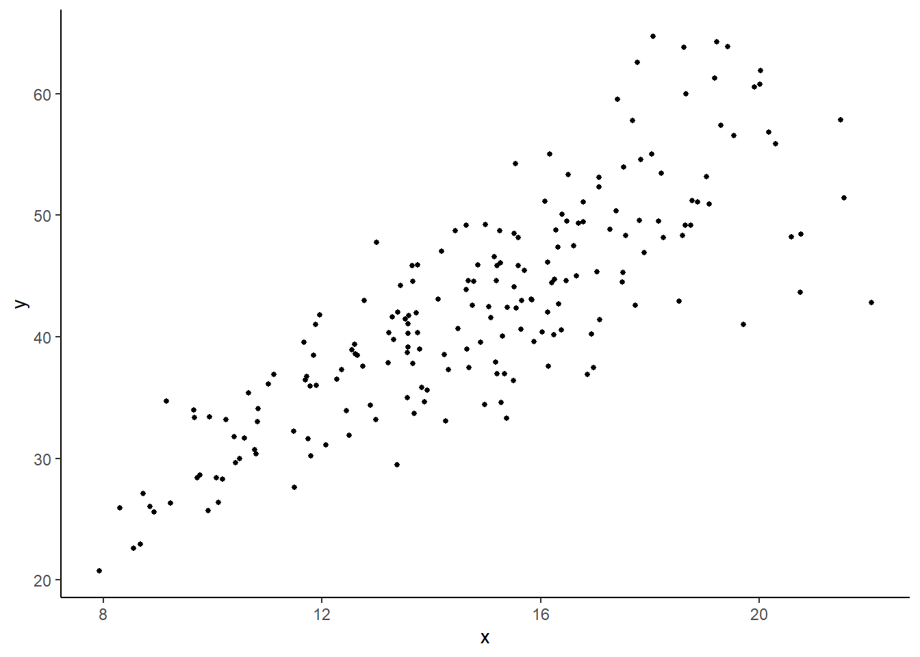
OLS estimation of this regression gives the following output.
ols <- lm(y~x, data=df_het)
sum_ols <- summary(ols)
coef(sum_ols)
cat("R-squared: ",sum_ols$r.squared,"\n")
Estimate Std. Error t value Pr(>|t|)
(Intercept) 6.285792 1.7817576 3.52786 5.207066e-04
x 2.430744 0.1177712 20.63955 3.034896e-51
R-squared: 0.6826877 Because there is obvious heteroskedasticity in this example, we should not trust the standard errors, t-statistics and p-values presented above. If we wish to stick with OLS, then we have to calculate the heteroskedasticity-robust standard error, which we do below using the vcovHC() function from the sandwich package. The heteroskedasticity-robust standard errors are the square root of the diagonal elements of the matrix rbst_V in the example below.
rbst_V <- sandwich::vcovHC(ols, type="HC0")
rbst_se <- sqrt(diag(rbst_V))
rbst_output <- coef(sum_ols)
colnames(rbst_output) <- c("Estimate", "rbst-se", "rbst-t", "p-val")
rbst_output[,'rbst-se'] <- rbst_se
rbst_output[,'rbst-t'] <- rbst_output[,'Estimate']/rbst_se
rbst_output[,'p-val'] <- 2*(1-pt(abs(rbst_output[,'rbst-t']),sum_ols$df[2]))
round(rbst_output,6)
Estimate rbst-se rbst-t p-val
(Intercept) 6.285792 1.863926 3.372339 0.000896
x 2.430744 0.136242 17.841435 0.000000Now we assume that \(\mathit{Var}(\epsilon_i \mid X) = \sigma^2X_i^2\), which seems reasonable given the scatterplot in Fig. 7.2. We run WLS using the weights option in lm() function. Note that the option weights refer to weights on the squared residuals, as in the \(\omega_{i}\) in (7.9), i.e., it is \(1/\eta_i\) if \(\sigma_i^2 = \sigma^2 \eta_i\).
df_het$wt <- 1/df_het$x^2
wls2 <- lm(y~x,data=df_het, weights=wt)
sum_wls2 <- summary(wls2)
coef(sum_wls2)
cat("R-squared: ", sum_wls2$r.squared,"\n")
Estimate Std. Error t value Pr(>|t|)
(Intercept) 4.82571 1.4065451 3.430896 7.321779e-04
x 2.53166 0.1023702 24.730430 1.839271e-62
R-squared: 0.755433 The standard errors are lower than in the OLS regression, which is not unexpected. Note that the \(R^2\) reported above is not the \(R_{wls}^2\) that was recommended in (7.10). We calculate \(R_{wls}^2\) below
ehat <- df_het$y - coef(wls2)[1] - coef(wls2)[2]*df_het$x
rss <- sum(ehat^2)
tss <- sum((df_het$y - mean(df_het$y))^2)
R2 <- 1 - rss/tss
cat("R-square: ", R2,"\n")
R-square: 0.6814966 We see that \(R_{wls}^2\) is lower than in the OLS regression, as expected, but only slightly so. The \(R^2\) provided by lm() when using weights is a “weighted R-squared”, obtained in the following way: let \(\overline{Y}_{wls}\) be the WLS estimator (with the same weights as previously) of \(\beta_0\) from the regression \(Y_i = \beta_0 + \epsilon_i\). In other words, \(\overline{Y}_{wls}\) is the weighted mean of \(\{Y_i\}_{i=1}^N\). Then \[
\text{weighted-}R^2
=
\frac{\sum_{i=1}^N w_i(\hat{Y}_{i}^{wls} - \overline{Y}_{wls})^2}
{\sum_{i=1}^N w_i(Y_{i}^{wls} - \overline{Y}_{wls})^2}\;.
\] In other words, it is the weighted fitted sum of squares divided by the weighted total sum of squares, centered on the weighted mean of \(\{Y_i\}_{i=1}^N\). We replicate the lm() weighted R-squared below:
wls0 <- lm(y~1, data=df_het, weights=wt)  # Regression on intercept only
tss_wtd <- sum(df_het$wt * (df_het$y - coef(wls0))^2)
fss_wtd <- sum(df_het$wt*(wls2$fitted.values - coef(wls0))^2)
WeightedR2 <- fss_wtd/tss_wtd
WeightedR2
[1] 0.755433One difficulty with WLS is that we generally do not know the form of the heteroskedasticity. In the simple linear regression case, should \(\eta_i\) be \(|X_{i1}|\) or \(X_{i1}^2\) or some other function of the regressors? The problem of specifying the form of the heteroskedasticity becomes more challenging in the multivariate regression case \[ Y_i = \beta_0 + \beta_1 X_{1,i} + \dots + \beta_{K-1,i}X_{K-1,i} + \epsilon_i\,,i=1, \dots, n\,. \] Any heteroskedasticity is likely to depend on more than one regressor, to different degrees, so there will be parameters to estimate. E.g., we might have something like \[ \eta_i = \exp(\alpha_1 X_{i1} + \dots + \alpha_{K-1} X_{i,K-1}) \] (the exponentiation is to ensure the variance is positive). Then to implement WLS, we first have to estimate the parameters in the variance equation. One way to do this is to first estimate the main equation using OLS, and obtain the OLS residuals. Then regress the log of the squared residuals on a constant and the regressors to estimate \(\sigma^2\) and the \(\alpha\) parameters, and then finally compute the “fitted variances” \(\widehat{\sigma_i^2}\) and weight the squared residuals by \(1/\widehat{\sigma_i^2}\).
7.3.2 Testing for Heteroskedasticity
It may be of interest to test whether heteroskedasticity is an issue in the first place. The following are some possible tests. All involve first estimating the main regression by OLS and obtaining the OLS residuals \(\hat{\epsilon}_{i,ols}\). First, run the regression \[ \hat{\epsilon}_{i, ols}^2 = \alpha_0 + \alpha_1X_{i1} + \dots \alpha_{K-1}X_{i,K-1}+u_i \] and test \(H_{0}: \alpha_1 = \dots = \alpha_{K-1}=0\) using an F test. An alternative is to use an “LM” test after running the regression above: under the null hypothesis, we have \[ NR_{\epsilon}^2 \; \overset{a}{\sim} \; \chi^2(K). \]
To allow for possible non-linear forms we can include powers of regressors and interaction terms between them in the variance regression: \[ \begin{aligned} \hat{\epsilon}_{i, ols}^2 = \alpha_0 &+ \alpha_1X_{i1} + \dots + \alpha_{K-1}X_{i,K-1} + \delta_1X_{i1}^2 + \dots + \delta_{K-1}X_{i,K-1}^2 + \gamma_{12} X_{i1}X_{i2} + \dots + u_i \end{aligned} \] then testing if all of the coefficients (not including the intercept) are zero. Obviously you lose degrees of freedom quickly as the number of regressors grow. One way around this problem is to run the regression \[ \hat{\epsilon}_{i, ols}^2 = \alpha_0 + \alpha_1\hat{Y}_{i,ols} + \alpha_{2}\hat{Y}_{i,ols}^2 + u_i \] where \(\hat{Y}_{i,ols}\) refers to the OLS fitted values from the main equation. The hypothesis that there is no heteroskedasticity is \(H_0: \alpha_1 = \alpha_2 = 0\) using an F test or an LM test.
The first approach is often referred to as Breusch-Pagan tests for heteroskedasticity. The approach using OLS fitted values is called the White test for heteroskedasticity.
Example 7.3 We apply the Breusch-Pagan test for heteroskedasticity to the regression \[ \ln earn = \beta_0 + \beta_1 \ln wexp_i + \beta_2 \ln tenure_i + \epsilon_i. \]
mdl <- lm(log(earn)~log(wexp)+log(tenure), data=df_earn)  #--Main Equation
cat("Main Regression\n")                            #--Main Regr Output Title
round(summary(mdl)$coefficients,4)                  #--Main Regr Output
Main Regression
Estimate Std. Error t value Pr(>|t|)
(Intercept) 2.9167 0.0229 127.3595 0
log(wexp) -0.0411 0.0095 -4.3294 0
log(tenure) 0.1746 0.0091 19.1215 0df_earn$ehat <- residuals(mdl) #--Get OLS Residuals
heteq <- lm((ehat^2)~log(wexp)+log(tenure), data=df_earn) #--BP-Test Regression
cat("Heteroskedasticity Test Regression\n") #--Test Regr Output Title
round(summary(heteq)$coefficients,4) #--Test Regr OutputHeteroskedasticity Test Regression
Estimate Std. Error t value Pr(>|t|)
(Intercept) 0.4668 0.0261 17.9070 0.0000
log(wexp) -0.0224 0.0108 -2.0728 0.0382
log(tenure) -0.0167 0.0104 -1.6028 0.1090## BP, F-version
f_het <- summary(heteq)$fstatistic #--Retrieve F-Stat (stat, df1, df2)
cat("BP-F Stat: ", f_het[1], " p-val: ", 1-pf(f_het[1], f_het[2], f_het[3]), "\n") BP-F Stat: 4.291278 p-val: 0.01373845 ## BP, LM-version
lm_het <- nobs(heteq)*summary(heteq)$r.squared # Calc. LM Stat.
lm_pval <- 1 - pchisq(lm_het, 2) # 2 restrictions
cat("BP-LM Stat: ", lm_het, " p-val: ", lm_pval, "\n", sep="")BP-LM Stat: 8.57288 p-val: 0.0137538There is some evidence of heteroskedasticity, and the individual t-tests suggest that the noise variance decreases with work experience.
7.4 Misspecification of Conditional Expectation
If you specify that \(E(Y \mid X_1) = \beta_0 + \beta_1 X_1\) but the conditional expectation does not have this form, then parameters become hard to interpret, if not meaningless, and predictions from the model will usually be biased. Fortunately, as we have seen, the multiple linear regression model provides one with substantial flexibility in specify the functional form, by transforming variables (including transforming the dependent variable), adding quadratic terms, using piecewise linear or piecewise quadratic forms, adding interaction terms, and many other possibilities. Of course, it may well be that the conditional expectation cannot be written in linear-in-parameters form, but often the multiple linear regression framework provides sufficient flexibility to at least get what appears to be an appropriate specification.
As a rough check for functional form adequacy, one can always plot residuals against individual regressors. If the functional specification is adequate, the residuals should look like random noise. For instance, if \(E(Y \mid X) = \beta_0 + \beta_1 X_1 + \beta_2 X_1^2\) but you specify \(E(Y \mid X) = \beta_0 + \beta_1 X_1\), then the residuals will display a quadratic pattern with respect to \(X_1\). Two more formal checks for functional form adequacy include the RESET test and tests of non-nested alternatives.
7.4.1 RESET test for functional form misspecification
Given a regression specification \[ Y_i = \beta_{0} + \beta_{1} X_{i1} + \dots + \beta_{K-1} X_{i,K-1} + \epsilon_i\,, \] the Regression Equation Specification Error Test (or “RESET Test”) checks if adding powers (\(X_{1,i}^2\), \(X_{2,i}^2\),…) and interaction terms (\(X_{1,i}X_{2,i}\), \(X_{1,i}X_{3,i}\), etc.) of the regressors can significantly improve the fit. Of course, this can lead to severe loss of degrees-of-freedom, and may cause multicollinearity issues. The trick employed by the RESET test is to add the squares, cubes, and possibly higher powers of the original OLS fitted values \(\hat{Y}_{i,ols}\) into the regression specification and tests if these additions have significant explanatory power. For instance, the squared fitted value is a linear combination of the squares of all the regressions and the interaction terms between them, so the hope is that if the squares of some of the regressors are important, this will get reflected as a significant coefficient on \(\widehat{Y}_{i, ols}^2\) when it is added to the test equation. The test equation is \[ Y_i = \beta_{0} + \beta_{1} X_{i1} + \dots + \beta_{K-1} X_{i,K-1} + \alpha_2\hat{Y}_{i,ols}^2 + \dots + \alpha_p\hat{Y}_{i,ols}^p + \epsilon_i\,, \tag{7.11}\] and the hypothesis of adequacy of the functional form specification is \[ H_0: \alpha_2 = \dots = \alpha_p = 0. \] The test equation cannot include \(\hat{Y}_{i,ols}\) (see exercises), and often only the second or second and third powers are included. An F-test (or t-test, if only the second power is included) can be used to test the hypothesis. We illustrate the RESET test in the next example. Note that the RESET test is interpreted as a test of adequacy of the functional form specification of the original regression, and not as saying anything about the whether or not certain variables should or should not be included.
Example 7.4 We apply the RESET test to the regression \[
\ln earn_i = \beta_0 + \beta_1 wexp_i + \beta_2 tenure_i + \epsilon_i.
\] using data in earnings2019.csv.
mdl_base <- lm(log(earn)~wexp+tenure, data=df_earn)
df_earn$yhat <- fitted(mdl_base)
mdl_test <- lm(log(earn)~wexp+tenure+I(yhat^2), data=df_earn)
cat("Base Regression:\n")
round(summary(mdl_base)$coefficients, 4)
cat("\nTest Regression:\n")
round(summary(mdl_test)$coefficients, 4)
Base Regression:
Estimate Std. Error t value Pr(>|t|)
(Intercept) 3.0249 0.0156 194.1339 0
wexp -0.0049 0.0011 -4.3724 0
tenure 0.0187 0.0011 17.1674 0
Test Regression:
Estimate Std. Error t value Pr(>|t|)
(Intercept) 17.3285 2.3951 7.2350 0
wexp -0.0531 0.0082 -6.5134 0
tenure 0.2092 0.0319 6.5528 0
I(yhat^2) -1.5680 0.2625 -5.9722 0The hypothesis of adequacy of the functional form in the base regression is rejected.
7.4.2 Testing Nonnested Alternatives
Regression specifications such as \[ \begin{aligned} &\text{[A]} \quad Y_i = \beta_0 + \beta_1X_{i1} + \beta_2 X_{i2} + \epsilon_i \\[1.5ex] \text{and} \quad &\text{[B]} \quad Y_i = \beta_0 + \beta_1\ln X_{i1} + \beta_2 \ln X_{i2} + \epsilon_i \end{aligned} \] are “non-nested alternatives”, i.e., one is not a special case of the other. One way of testing which specification fits better is to construct a “super-model” that includes both [A] and [B] as restricted cases, i.e., \[ \text{[A]} \quad Y_i = \beta_0 + \beta_1X_{i1} + \beta_2 X_{i2} + \beta_3 \ln X_{i1} + \beta_4 \ln X_{i2} + \epsilon_i \] and to test for coefficient significance. This approach is often plagued by multicollinearity problems. An alternative is to fit both models separately, collect their fitted values, and include each fitted value series as a regressor in the other specification, i.e., regress \[ \begin{aligned} &\text{[A']} \quad Y_i = \beta_0 + \beta_1X_{i1} + \beta_2 X_{i2} + \delta_1 \hat{Y}_i^B + \epsilon_i \\[1.5ex] \text{and} \quad &\text{[B']} \quad Y_i = \beta_0 + \beta_1\ln X_{i1} + \beta_2 \ln X_{i2i} + \delta_2 \hat{Y}_i^A + \epsilon_i \end{aligned} \] and test (separately) if the coefficients on the fitted values are statistically significant. The idea is to see if each specification has anything to add to the other. If \(\delta_1=0\) is rejected and \(\delta_2=0\) is not, then this suggests that [B] is a better specification (the result does not suggest [B] is the best specification, just better than [A].) Likewise, [A] is preferred to [B] if \(\delta_2=0\) is rejected and \(\delta_1=0\) is not. It may be that both are rejected, which suggests that neither specification is adequate. If neither are rejected, then it appears that there is little in the data to distinguish between the two specifications. Note that the dependent variable in both alternatives must be the same.
We compare the specifications \[ \begin{aligned} &\text{[A]} \quad \ln earn_i = \beta_0 + \beta_1 wexp_i + \beta_2 tenure_i + \epsilon_i \\ \text{and} \quad &\text{[B]} \quad \ln earn_i = \beta_0 + \beta_1 \ln wexp_i + \beta_2 \ln tenure_i + \epsilon_i\,. \end{aligned} \]
mdlA <- lm(log(earn)~wexp+tenure, data=df_earn)
mdlB <- lm(log(earn)~log(wexp)+log(tenure), data=df_earn)
df_earn$yhatA <- fitted(mdlA)
df_earn$yhatB <- fitted(mdlB)
cat("Model A plus yhatB:\n")
mdlAplusB <- lm(log(earn)~wexp+tenure+yhatB, data=df_earn)
round(summary(mdlAplusB)$coefficients,4)
cat("\nModel B plus yhatA:\n")
mdlBplusA <- lm(log(earn)~log(wexp)+log(tenure)+yhatA, data=df_earn)
round(summary(mdlBplusA)$coefficients,4)
Model A plus yhatB:
Estimate Std. Error t value Pr(>|t|)
(Intercept) 0.2825 0.3331 0.8482 0.3963
wexp -0.0012 0.0012 -0.9975 0.3186
tenure 0.0022 0.0023 0.9532 0.3406
yhatB 0.9075 0.1101 8.2430 0.0000
Model B plus yhatA:
Estimate Std. Error t value Pr(>|t|)
(Intercept) 2.5557 0.3606 7.0876 0.0000
log(wexp) -0.0373 0.0103 -3.6330 0.0003
log(tenure) 0.1577 0.0192 8.2204 0.0000
yhatA 0.1219 0.1215 1.0033 0.3158It appears that the specification [B] is preferred over specification [A].
7.5 Omitted Variables
We have already discussed the problem of omitted variables at length. Basically the problem is that you estimate \[ E(Y \mid X_1, \dots, X_{K-1}) = \beta_0 + \beta_1 X_1 + \dots + \beta_{K-1}X_{K-1} \tag{7.12}\] when you really want to be estimating \[ \begin{aligned} E(Y &\mid X_1, \dots, X_{K-1}, X_{K}, \dots, X_{M}) \\ &= \beta_0 + \beta_1 X_1 + \dots + \beta_{K-1}X_{K-1} +\beta_K X_{K} + \dots + \beta_{K+M}X_{K+M}\,. \end{aligned} \tag{7.13}\] Maybe there are factors \(X_1, \dots, X_{M}\) that directly affect \(Y\). You are interested in the direct effect of \(X_1\) on \(Y\), and you think to control for the factors \(X_2\), \(\dots\), \(X_{K-1}\), but not the others. If there are correlations between the omitted variables \(X_{K}, \dots, X_{M}\) and the included variables \(X_1, \dots, X_{K-1}\), then the coefficients on \(X_1, \dots, X_{K-1}\) in (7.12) will generally not be the same as the coefficients on \(X_1, \dots, X_{K-1}\) in (7.13), including the parameter \(\beta_1\) of particular interest. If none of the variables in \(X_{K}, \dots, X_{M}\) are correlated with any of the variables in \(X_1, \dots, X_{K-1}\), then the coefficients on \(X_1, \dots, X_{K-1}\) in (7.12) will be the same as the coefficients on \(X_1, \dots, X_{K-1}\) in (7.13), but even then, including the omitted variables will usually help reduce standard errors.
The solution to the omitted variable problem is, of course, to include the missing variables, but this assumes that the missing variables are available. In applications, often we want to include variables in a regression that are simply not available, or perhaps of low quality. As an example, in the returns to schooling equation \[ \ln earn = \beta_0 + \beta_1 educ + \text{(controls)} + \epsilon \] Controls may include race and sex variables, tenure, age, etc. One control one would like to put in would be some measure of innate ability, but this is a notoriously difficult variable to estimate, an proxies such as IQ or grades may not even be available for the individuals in your sample.
There are a few solutions available (depending on the specifics of the problem, structure of the data, etc.). One solution is to use “instrumental variables” and “instrumental variable estimation”. We explore this in the next chapter.
7.6 Sampling issues
So far we have assumed an iid random sample from the population. The problems we have discussed arise from misspecification issues (e.g., omitted variables, incorrect function form for the conditional expectation). Now we consider two examples where you may have the correct specification, but sampling issues lead to biased estimates.
7.6.1 Truncated Sampling
Consider the simple linear regression \[ Y_i = \beta_0 + \beta_1 X_{i1} + \epsilon_i \] and suppose \(\beta_1\) is positive so you have a positively sloped PRF. Suppose you have a “truncated sample” where you cannot observe any observation where \(Y_i > c\). This means that the only observations with larger values of \(X_i\) that are included in your sample will be the ones with lower or negative values of \(\epsilon_i\), since a large \(X_{i1}\) together with large positive \(\epsilon_i\) makes \(Y_i>c\) more likely. This implies a negative correlation between \(X\) and \(\epsilon\), and invalidates the assumption \(E(\epsilon_{i} \mid X_{11}, \dots, X_{n1})=0\). The following is an empirical illustration where the PRF has a positive slope, and observations with \(Y_i>1500\) are unavailable. The plot in Fig. 7.3 shows the full (black circles) and truncated (red x’s) samples. The estimated OLS sample regression line for the full data set (black) and the truncated data set (red) are shown, illustrating the downward bias in \(\hat{\beta}_{1}\).
  set.seed(13)
  X <- rnorm(100, mean=50, sd=20)
  Y <- 1220 + 4*X + rnorm(100, mean=0, sd=50)
  df_notrunc <- data.frame(X, Y)
  df_trunc <- filter(df_notrunc, Y<=1500)
  ggplot() +
    geom_point(data=df_notrunc,aes(x=X,y=Y), pch=1, size=2) +
    geom_smooth(data=df_notrunc,aes(x=X,y=Y), method="lm", se=FALSE, col="black") +
    geom_point(data=df_trunc, aes(x=X,y=Y), pch=4, size=2,col='red') +
    geom_smooth(data=df_trunc,aes(x=X,y=Y), method="lm", se=FALSE, col="red") +
    theme_minimal()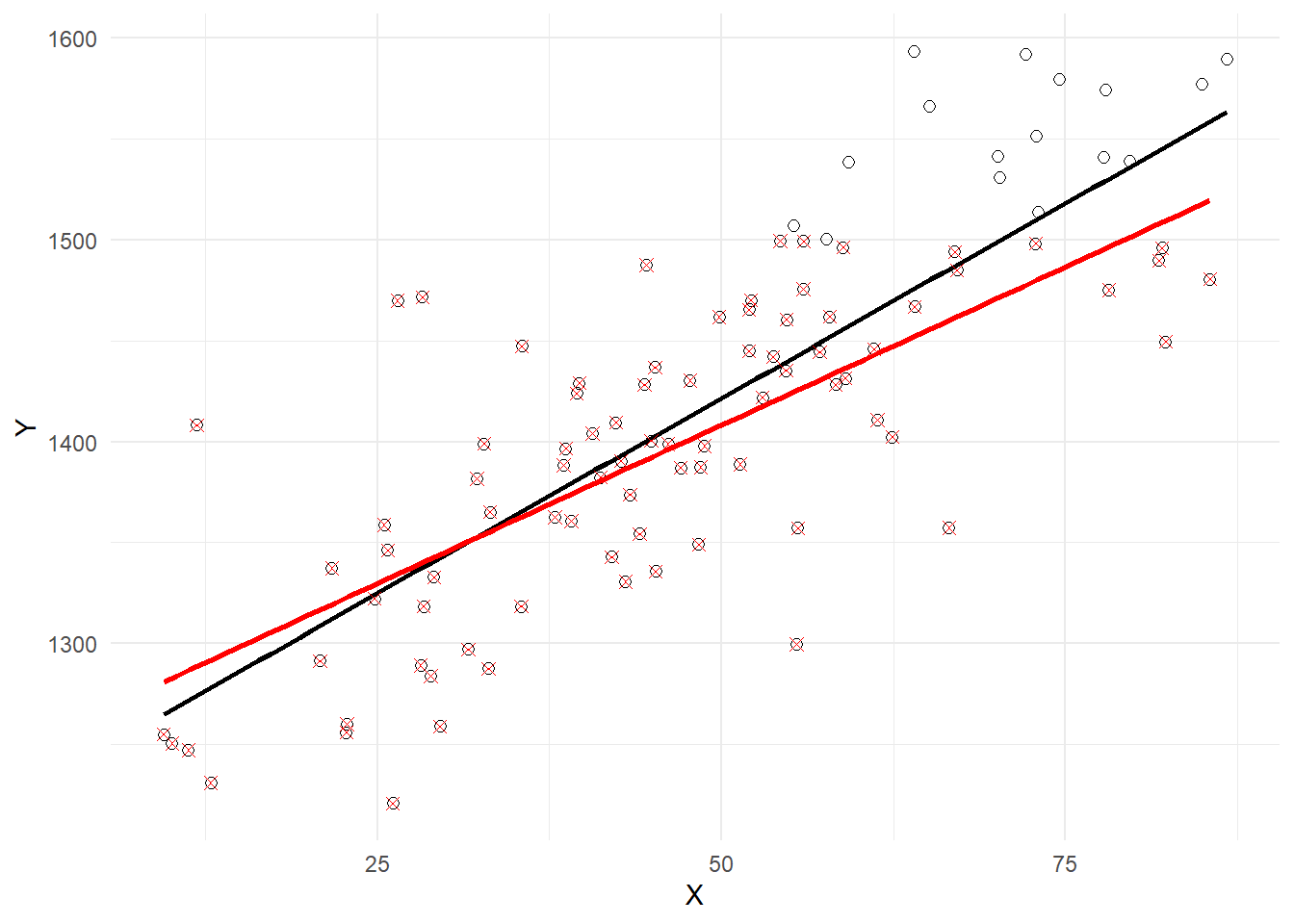
A related problem with similar outcome is censored sampling. Imagine, for instance, that the observations with \(Y\) above 1500 are not missing, but the actual value of \(Y\) is replaced with \(Y = 1500\). The solutions to this and the truncated sampling problem requires us to go beyond the least squares/linear regression framework, and is covered in the chapter on limited dependent variables.
7.6.2 Measurement Error
Another kind of sampling issue is measurement error. Suppose \(Y = \beta_0 + \beta_1 X + \epsilon\) describes the relationship between \(Y\) and \(X\), but \(X\) is only observed with error, i.e., you observe \(X^{*} = X + u\). Assume that the measurement error \(u\) is independent of \(X\). Then \[ \begin{aligned} Y &= \beta_0 + \beta_1 X + \epsilon \\ &= \beta_0 + \beta_1 (X^* - u) + \epsilon \\ &= \beta_0 + \beta_1 X^* + (\epsilon - \beta_1u) \\ &= \beta_0 + \beta_1 X^* + v \end{aligned} \] where \(v = \epsilon - \beta_1 u\). You proceed with what appears to be the only feasible option to you, which is to run the regression \[ Y = \beta_0 + \beta_1 X^* + v\,, \] but since \(u\) is correlated with \(X^*\), the assumption \(E[v|X^*]=0\) does not hold. In the simulated example below, we have a positively sloped PRF, shown in red, and measurement error in the regressor. Since \(\beta_1\) is positive, \(X^*\) and \(v\) are negatively correlated, meaning that the error term \(v\) will tend to be positive for smaller \(X*\) and negative for larger \(X*\). This tendency is visible in Fig. 7.4 below. The red circles are the sample you would have observed with no measurement error. The black circles are the same sample points, but with measurement error in the \(X_{i}\)’s.
  set.seed(13)
  X <- rnorm(100, mean=50, sd=20)
  Y <- 1220 + 4*X + rnorm(100, mean=0, sd=10)
  Xstar <- X + rnorm(100, mean=0, sd=10)
  df_measerr <- data.frame(X, Y, Xstar)
  ggplot() +
    geom_point(data=df_measerr,aes(x=Xstar,y=Y), pch=1, size=2) +
    geom_point(data=df_measerr,aes(x=X,y=Y), pch=1, size=2, col="red") +
    geom_abline(intercept=1220, slope=4, col='red') +
    geom_smooth(data=df_measerr, aes(x=Xstar, y=Y), method="lm", col='black',
                se=FALSE, linewidth=0.8) + xlab("X, Xstar") +
    theme_minimal()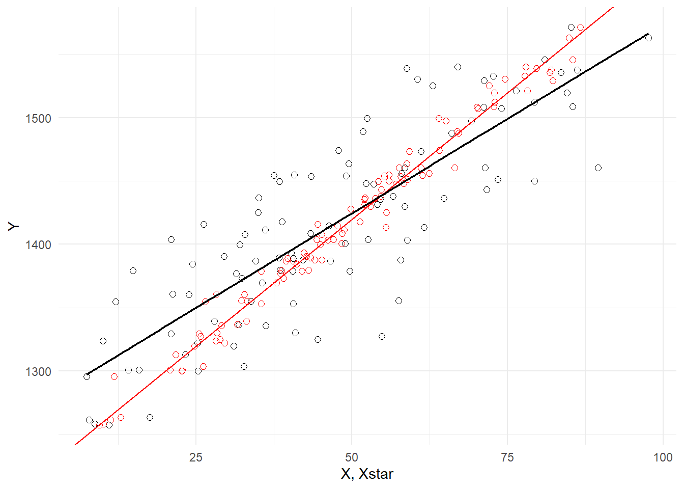
The instrumental variable approach covered in the chapter on that topic may be able to handle this problem.
7.7 Simultaneity Bias
Suppose now that we actually don’t want to estimate a conditional expectation, but we want instead to estimate a “structural equation”. Consider a demand-and-supply example. Suppose the market for a good is governed by the following demand and supply equations \[ \begin{aligned} Q_t^d &= \delta_0 + \delta_1 P_t + \epsilon_t^d \hspace{1cm} &(\text{Demand Eq } \delta_1 < 0) \\ Q_t^s &= \alpha_0 + \alpha_1 P_t + \epsilon_t^s \hspace{1cm} &(\text{Supply Eq } \alpha_1 > 0) \\ Q_t^s &= Q_t^d \hspace{3cm} &(\text{Market Clearing}) \end{aligned} \] where \(Q\) and \(P\) represent log quantities and log prices respectively, so \(\delta_1\) and \(\alpha_1\) represent price elasticities of demand and supply respectively. Suppose the demand shock \(\epsilon_t^d\) and supply shock \(\epsilon_y^s\) are iid noise terms with zero means and variances \(\sigma_d^2\) and \(\sigma_s^2\) respectively, and are mutually uncorrelated. Market clearing means that observed quantity and prices occur at the intersection of the demand and supply equations, i.e., observed prices are such that \[ \delta_0 + \delta_1 P_t + \epsilon_t^d = \alpha_0 + \alpha_1 P_t + \epsilon_t^s \] which we can solve to get \[ P_t = \frac{\alpha_0 - \delta_0}{\delta_1 - \alpha_1} + \frac{\epsilon_t^s - \epsilon_t^d}{\delta_1 - \alpha_1}. \tag{7.14}\] Substituting this expression for prices into either the demand or supply equation gives \[ Q_t = \left(\delta_0 + \delta_1\frac{\alpha_0 - \delta_0}{\delta_1 - \alpha_1}\right) + \frac{\delta_1\epsilon_t^s - \alpha_1\epsilon_t^d}{\delta_1 - \alpha_1}\,. \tag{7.15}\] Equations 7.14 and 7.15 imply \[ \mathit{Var}(P_t) = \frac{\sigma_s^2 + \sigma_d^2}{(\delta_1 - \alpha_1)^2} \quad \text{ and } \quad \mathit{Cov}(P_t, Q_t) = \frac{\delta_1\sigma_s^2 + \alpha_1\sigma_d^2}{(\delta_1 - \alpha_1)^2}. \] This means that in a regression of \(Q_t = \beta_0 + \beta_1 P_t + \epsilon_t\), we will get \[ \hat{\beta}_1 \overset{p}{\longrightarrow} \frac{\mathit{Cov}(Q_t, P_t)}{\mathit{Var}(P_t)} =\frac{\delta_1\sigma_s^2 + \alpha_1\sigma_d^2}{\sigma_s^2 + \sigma_d^2} \tag{7.16}\] which is neither the price elasticity of demand nor the price elasticity of supply, but a linear combination of the two.
Fig. 7.5 illustrates this issue. We simulate the demand and supply example with a series of random demand and supply shocks. Each demand shock shifts the demand curve and each supply shock shifts the supply curve resulting in a new intersection point. The set of equilibrium prices and quantity does not reflect either the demand or the supply function.
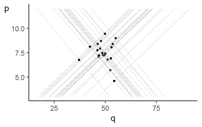
The problem here is that prices and quantities are simultaneously determined by the intersection of the demand and supply functions; both prices and quantities are “endogenous” variables. The consequence of this is that regardless of whether you view the regression of \(Q_t\) on \(P_t\) as estimating the demand or supply equation, the noise term in the regression will be correlated with \(P_t\). A supply shock shifts the supply function and changes both \(Q_t\) and \(P_t\). Likewise, a demand shock shifts the demand function and again changes both \(Q_t\) and \(P_t\). The use of the term “endogeneity” comes from applications like these, but it is now used for all situations where the noise term is correlated with one or more of the regressors.
7.8 Exercises
Exercise 7.1 Show that the OLS estimator (7.2) for \(\beta_1\) in Example 7.1 is unbiased. Show also that the modified noise terms are uncorrelated, i.e., \[ E(\epsilon_i^*\epsilon_j^* \mid X) = 0 \] for all \(i \neq j\); \(i,j=1,2,...,N\).
Exercise 7.2 In the notes we claimed that \[ \frac{\sum_{i=1}^N X_i^4}{\left(\sum_{i=1}^N X_i^2\right)^2} \geq \frac{1}{N}. \] Prove this by showing that for any set of values \(\{z_i\}_{i=1}^N\), we have \[ N\sum_{i=1}^N z_i^2 - \left( \sum_{i=1}^N z_i\right)^2 \geq 0. \] (Hint: start with the fact that \(\sum_{i=1}^N(z_i - \bar{z})^2 \geq 0\).) Then substitute \(X_i^2\) for \(z_i\). When will equality hold?
Exercise 7.3
Calculate the heteroskedasticity-robust standard errors for the regression in Example 7.3. Compare the robust standard errors with the OLS standard errors.
Estimate (using
lm()) the main equation in Example 7.3 using WLS, assuming \[ \mathit{Var}(\epsilon_i \mid \{wexp\}_{i=1}^n, \{tenure\}_{i=1}^n) = \sigma^2 wexp_i\,. \] Compare the WLS estimation results with the OLS estimation results (with heteroskedasticity robust standard errors).
Exercise 7.4
Why is it that we cannot include \(\hat{Y}_{i,ols}\) in the RESET test equation?
Add the third power of the OLS fitted value in the RESET test equation in Example 7.4. What happens to the statistical significance of the original regressors? Can you explain the likely cause? Hint: what is the correlation between
yhat^2andyhat^3?
Exercise 7.5 We have shown that measurement error in the regressor leads to inconsistent estimators. Does measurement error in the regressand \(Y\) also result in inconsistent estimators?
Unfortunately, default standard errors in virtually all econometric software libraries are based on the homoskedastic version of the variance-covariance matrix of \(\widehat{\beta}^{ols}\).↩︎