3 Conditional Expectations / Linear Regression Overview

We will use the following packages in these notes:

library(tidyverse)
library(patchwork)
library(latex2exp)

3.1 Joint and Conditional Probabilities

We model the joint behavior of two random variable using a joint probability distribution function. We will use a simple example with two discrete random variables to illustrate the main ideas.

3.1.1 Joint and Marginal Distributions

Suppose \(X\) and \(Y\) are discrete random variables with range \(x=1,2,3,4,5\) and \(y=3.0, 3.5, 4.0, 4.5, 5.0, 5.5, 6.0\). Their joint pdf \(f_{X,Y}(x,y)\) gives you the probability of events of the form \(X=x\) and \(Y=y\), i.e., \[ f_{X,Y}(x,y) = \Pr(X=x, Y=y)\,. \] Suppose the joint pdf of \(X\) and \(Y\) are as given below:

\[ \begin{array}{@{}cc|ccccc@{}} & 6 & 0 & 0 & 0 & 0 & \frac{1}{20} \\ & 5.5 & 0 & 0 & 0 & \frac{1}{20} & \frac{2}{20} \\ & 5 & 0 & 0 & \frac{1}{20} & \frac{2}{20} & \frac{1}{20} \\ y & 4.5 & 0 & \frac{1}{20} & \frac{2}{20} & \frac{1}{20} & 0 \\ & 4 & \frac{1}{20} & \frac{2}{20} & \frac{1}{20} & 0 & 0 \\ & 3.5 & \frac{2}{20} & \frac{1}{20} & 0 & 0 & 0 \\ & 3 & \frac{1}{20} & 0 & 0 & 0 & 0 \\ \hline & & 1 & 2 & 3 & 4 & 5 \\ & & & & x & & \end{array} \tag{3.1}\] so we have, for example, \[ \Pr(X=1,Y=3)=f_{X,Y}(1,3) = \frac{1}{20}, \Pr(X=3,Y=3)=0, \Pr(X\geq 4,Y\geq 5)= \frac{7}{20} \,. \] In a large sample of observations \(\{X_i, Y_i\}_{i=1}^n\) from this population, you should find that approximately 1/20th of the observations will comprise the pair \((X_i, Y_i) = (1,3)\), approximately 35% of the sample will have \(X_i \geq 4\) and \(Y_i \geq 5\), and will be no observations with \(X_i=3\) and \(Y_i=3\).

What is the probability of observing \(X=1\) (regardless of the value of the accompanying \(Y\) value)? To find \(\Pr(X=1)\), add up all the probabilities of events where \(X=1\), i.e., \[ \begin{aligned} \Pr(X=1) &= \Pr(Y=3,X=1)+\Pr(Y=3.5,X=1)+\cdots+\Pr(Y=6,X=1) \\ &= \frac{1}{20} + \frac{2}{20} + \frac{1}{20} = 0.2\,. \end{aligned} \] You can repeat this calculation for \(\Pr(X=2)\), \(\Pr(X=3)\), \(\Pr(X=4)\), \(\Pr(X=5)\). You should find that: \[ \begin{array}{@{}c|ccccc@{}} x & 1 & 2 & 3 & 4 & 5 \\ \hline \Pr(X=x) & \frac{4}{20} & \frac{4}{20} & \frac{4}{20} & \frac{4}{20} & \frac{4}{20} \end{array} \] This is the “marginal” (or “unconditional”) pdf of \(X\). In this example \(X\) is uniformly distributed over the values \(X = 1,2,...,5\). If you look at a large sample of observations \(\{X_i, Y_i\}_{i=1}^n\) from this population, you will find that 1/5th of the pairs \((X_i, Y_i)\) in your sample will have \(X_i = 1\), 1/5th will have \(X_i = 2\) and so on.

Similar calculations will give you the marginal distribution of \(Y\).

\[ \begin{array}{@{}ccccc@{}} \begin{array}{@{}cc|ccccc@{}} & 6 & 0 & 0 & 0 & 0 & \frac{1}{20} \\ & 5.5 & 0 & 0 & 0 & \frac{1}{20} & \frac{2}{20} \\ & 5 & 0 & 0 & \frac{1}{20} & \frac{2}{20} & \frac{1}{20} \\ y & 4.5 & 0 & \frac{1}{20} & \frac{2}{20} & \frac{1}{20} & 0 \\ & 4 & \frac{1}{20} & \frac{2}{20} & \frac{1}{20} & 0 & 0 \\ & 3.5 & \frac{2}{20} & \frac{1}{20} & 0 & 0 & 0 \\ & 3 & \frac{1}{20} & 0 & 0 & 0 & 0 \\ \hline & & 1 & 2 & 3 & 4 & 5 \\ & & & & x & & \end{array} &\rightarrow &\begin{array}{@{}c|c@{}} 6 & \frac{1}{20} \\ 5.5 & \frac{3}{20} \\ 5 & \frac{4}{20} \\ 4.5 & \frac{4}{20} \\ 4 & \frac{4}{20} \\ 3.5 & \frac{3}{20} \\ 3 & \frac{1}{20} \\ \hline y & \Pr(Y=y) \\ & \end{array} &\rightarrow &\begin{array}{rcl} E(Y) &= &4.5 \\ \mathit{Var}(Y) &= &0.625 \end{array} \\ \qquad\qquad \downarrow & & & & \\ \,\,\begin{array}{@{}c|ccccc@{}} x & 1 & 2 & 3 & 4 & 5 \\ \hline \Pr(X=x) & \frac{4}{20} & \frac{4}{20} & \frac{4}{20} & \frac{4}{20} & \frac{4}{20} \end{array} &\rightarrow &E(X)=3, \mathit{Var}(X)=2 & & \end{array} \]

The marginal distribution of \(Y\) in our example is somewhat “bell-shaped”. You can calculate the (unconditional) means and variances of \(X\) and \(Y\) from their marginal pdfs using the usual formulas.

In general, the joint pdf of two random variables is the function \(f_{X,Y}(x,y)\). For discrete random variables, the marginal pdf of \(X\) is computed as \(f_X(x) =\sum_y f_{X,Y}(x,y)\) where \(\sum_y\) indicates summation over the possible values of \(Y\). Likewise, the marginal pdf of \(Y\) is computed as \(f_Y(y) =\sum_x f_{X,Y}(x,y)\). For continuous random variables, the marginals are computed as integrals: \[ f_X(x) =\int_Y f_{X,Y}(x,y)\,dy \; \text{ and } \; f_Y(y) =\int_X f_{X,Y}(x,y) \, dx\,. \] We can extend the joint pdf concept to multiple variables, e.g., \(f_{X,Y,Z}(x,y,z)\), and so on.

3.1.2 Covariance and Correlation

It seems clear from (3.1) that there is a positive relationship between \(X\) and \(Y\). One way to describe the relationship between the random variables is to calculate the covariance between \(X\) and \(Y\), defined as \[ \sigma_{X,Y} = \mathit{Cov}(X,Y) = E((X-E(X))(Y-E(Y))). \] In our example, we have

\[ \begin{aligned} \mathit{Cov}(X,Y) = \;&(5-3)(6.0-4.5)\tfrac{1}{20} + \\ &(4-3)(5.5-4.5)\tfrac{1}{20} + (5-3)(5.5-4.5)\tfrac{2}{20} + \\ &(3-3)(5.0-4.5)\tfrac{1}{20} + (4-3)(5.0-4.5)\tfrac{2}{20} + (5-3)(5.0-4.5)\tfrac{1}{20} + \\ &(2-3)(4.5-4.5)\tfrac{1}{20} + (3-3)(4.5-4.5)\tfrac{2}{20} + (4-3)(4.5-4.5)\tfrac{1}{20} + \\ &(1-3)(4.0-4.5)\tfrac{1}{20} + (2-3)(4.0-4.5)\tfrac{2}{20} + (3-3)(4.0-4.5)\tfrac{1}{20} + \\ &(1-3)(3.5-4.5)\tfrac{2}{20} + (2-3)(3.5-4.5)\tfrac{1}{20} + \\ &(1-3)(3.0-4.5)\tfrac{1}{20} \\ = \;&1 \end{aligned} \] One problem with the covariance measure is that it is not invariant to scale. For instance, suppose \(X\) is currently measured in thousands of dollars. If we re-scale to dollars by multiplying \(X\) by 1000, then the covariance becomes \[ \begin{aligned} \mathit{Cov}(1000X,Y) &= E((Y-E(Y))(1000X-E(1000X))) \\ &= 1000E((Y-E(Y))(X-E(X))) \\ &= 1000 \mathit{Cov}(X,Y). \end{aligned} \] For this reason, the correlation coefficient \[ \rho_{X,Y} = \mathit{Corr}(X,Y) = \frac{\mathit{Cov}(X,Y)}{\sqrt{\mathit{Var}(X)}\sqrt{\mathit{Var}(Y)}}, \] which is invariant to scale and always lies between \(-1\) and \(1\), is more informative.

Given a sample \(\{X_i, Y_i\}_{i=1}^{n}\) from a joint pdf \(f_{X,Y}(x,y)\), we can estimate the covariance using the sample covariance \[ \widehat{\sigma}_{X,Y} = \frac{1}{n-1}\sum_{i=1}^{n}(X_i-\overline{X})(Y_i-\overline{Y}) \] where \(\overline{X}\) and \(\overline{Y}\) are the sample means of \(X_i\) and \(Y_i\) respectively. To estimate the correlation coefficient, we can divide the sample covariance by the sample standard deviations, i.e., \[ \widehat{\rho}_{X,Y} = \frac{\sum_{i=1}^{n}(X_i-\overline{X})(Y_i-\overline{Y})} {\sqrt{\sum_{i=1}^{n}(X_i-\overline{X})^2}\sqrt{\sum_{i=1}^{n}(Y_i-\overline{Y})^2}}\;\;. \] The following properties of means, variances and covariances are easy to show: if \(a\) and \(b\) are constants, we have

\(E(aX + bY) = aE(X) + bE(Y)\),
\(\mathit{Var}(aX+bY) = a^2\mathit{Var}(X) + b^2\mathit{Var}(Y) + 2ab\mathit{Cov}(X,Y)\),
\(\mathit{Cov}(X,Y) = E(XY) - E(X)E(Y)\),
\(\mathit{Cov}(X,X) = \mathit{Var}(X)\).

From ii, we see that the variance of a sum is the sum of the variances only if the variables are uncorrelated. From iii we see that \(\mathit{Cov}(X,Y) = E(XY)\) if either \(X\) or \(Y\) has mean zero.

3.1.3 Conditional Distributions

Another way of describing the relationship between random variables is via conditional distributions. These describe the behavior of one variable for various values of the other. For instance, if we observe \(X=1\) but do not observe the \(Y\) realization, what can we predict about the behavior of \(Y\)? For the joint pdf in (3.1), we know that only three values of \(Y\) are possible when \(X=1\), with \(Y=1\) and \(Y=4\) equally likely, and \(Y=3.5\) twice as likely as either of these. Other values of \(Y\) have probability zero. To describe the behavior of \(Y\) when \(X=1\) as a probability distribution function, we have to make the total probabilities when \(X=1\) sum to one, so we divide each of these probabilities by their sum (i.e., by \(\Pr(X=1)\)) to obtain the conditional probabilities:

\[ \begin{gathered} \Pr(Y=3 \mid X=1) = \frac{\frac{1}{20}}{\frac{4}{20}} = \frac{1}{4} \, , \, \Pr(Y=3.5 \mid X=1) = \frac{\frac{2}{20}}{\frac{4}{20}} = \frac{1}{2} \, , \, \Pr(Y=4 \mid X=1) = \frac{1}{4} \, , \\[2ex] \Pr(Y=4.5 \mid X=1) = \Pr(Y=5.5 \mid X=1) = \Pr(Y=6.5 \mid X=1) = 0\,. \end{gathered} \] This collection of probabilities make up the conditional pdf of \(Y\) given \(X=1\). Making these calculations for each value of \(X\) gives \[ \begin{gathered} \qquad\qquad\Pr(Y \mid X) \\ \begin{array}{@{}cc|ccccc@{}} & 6 & 0 & 0 & 0 & 0 & \frac{1}{4} \\ & 5.5 & 0 & 0 & 0 & \frac{1}{4} & \frac{1}{2} \\ & 5 & 0 & 0 & \frac{1}{4} & \frac{1}{2} & \frac{1}{4} \\ Y & 4.5 & 0 & \frac{1}{4} & \frac{1}{2} & \frac{1}{4} & 0 \\ & 4 & \frac{1}{4} & \frac{1}{2} & \frac{1}{4} & 0 & 0 \\ & 3.5 & \frac{1}{2} & \frac{1}{4} & 0 & 0 & 0 \\ & 3 & \frac{1}{4} & 0 & 0 & 0 & 0 \\ \hline & & 1 & 2 & 3 & 4 & 5 \\ & & & & X & & \end{array} \end{gathered} \tag{3.2}\] Each column of (3.2) represents a complete pdf, so we have a collection of five pdfs, one for each possible value of \(X\).

For any given value of \(X=x\), we can use the corresponding conditional pdf to compute the conditional mean of \(Y\) given \(X=x\), and the conditional variance of \(Y\) given \(X=x\). For \(X=1\), we have: \[ \begin{aligned} E(Y \mid X=1) &= 3(\tfrac{1}{4})+3.5(\tfrac{1}{2})+4(\tfrac{1}{4})+4.5(0)+5(0)+5.5(0)+6(0) = 3.5 \\ \mathit{Var}(Y \mid X=1) &= (3-3.5)^2(\tfrac{1}{4})+(3.5-3.5)^2(\tfrac{1}{2})+(4-3.5)^2(\tfrac{1}{4})+0+0+0+0 = 0.125 \end{aligned} \] Repeating these calculations for each value of \(X\) we get: \[ \begin{array}{@{}c|ccccc@{}} X & 1 & 2 & 3 & 4 & 5 \\ \hline E(Y \mid X) & 3.5 & 4 & 4.5 & 5 & 5.5 \\ \mathit{Var}(Y \mid X) & 0.125 & 0.125 & 0.125 & 0.125 & 0.125 \\ \end{array} \tag{3.3}\] Notice that \(E(Y \mid X)\) is a function of \(X\). In our example, the conditional mean of \(Y\) given \(X\) increases with \(X\). In particular, we have \(E(Y \mid X) = 3 + 0.5X\, , \, X = 1,2,3,4,5\). The conditional variance in this example turns out to be constant: \(\mathit{Var}(Y \mid X)=0.125\) for all \(X\). In general it may vary with \(X\).

In this example, knowledge of the value of \(X\) gives us information that we can use to refine our view of the behavior of \(Y\). For instance, if we know that \(X\) is small (relative to its mean), then we know that the mean of \(Y\) will also tend to be small (relative to its unconditional mean). If we know that the \(X\) is large, then we also know that the \(Y\) outcome will be large. If we do not observe \(X\), then our view regarding the mean value of \(Y\) will have to cover all possible values of \(X\), which is what the unconditional mean of \(Y\) does. The fact that \(X\) gives us information about \(Y\) is also reflected in the reduction in variance from \(\mathit{Var}(Y)=0.625\) to \(\mathit{Var}(Y \mid X)=0.125\). The inequality \(\mathit{Var}(Y \mid X) \leq \mathit{Var}(Y)\) does not hold in general, but it does hold when \(\mathit{Var}(Y \mid X)\) is constant.

For general continuous random variables, the conditional distributions can be computed as \[ f_{Y \mid X}(y \mid x) = \frac{f_{X,Y}(x,y)}{f_X(x)} \, \text{ and } \, f_{X \mid Y}(x \mid y) = \frac{f_{X,Y}(x,y)}{f_Y(y)} \] when \(f_Y(y) \neq 0\) and \(f_X(x) \neq 0\). Another way of writing this is \[ f_{X,Y}(x,y) = f_{Y \mid X}(y \mid x)f_X(x) = f_{X \mid Y}(x \mid y)f_Y(y). \]

This decomposition of joint pdfs can be extended to more than two variables, e.g., we have \[ f_{X,Y,Z}(x,y,z) = f_{Z \mid Y,X}(z \mid y,x)f_{Y \mid X}(y \mid x)f_{X}(x)\,. \]

3.1.4 Manipulating Conditional Moments

Manipulation of conditional expectations and variances follows one simple principle: whatever is being conditioned on can be treated as “fixed” (i.e., like a constant) as far as that expectation or variance is concerned.

Example 3.1

\(E(aXY \mid X) = aXE(Y \mid X) \, , \, \mathit{Var}(aXY \mid X) = a^2X^2\mathit{Var}(Y \mid X)\),

\(E(aX \mid X) = aX\) (contrast with \(E(aX)=aE(X)\), a constant),

\(\mathit{Var}(aX \mid X) = 0\) (contrast with \(\mathit{Var}(aX)=a^2\mathit{Var}(X)\)),

If \(Y = \beta_0 + \beta_1X + \epsilon\) with \(E(\epsilon \mid X)=0\) and \(\mathit{Var}(\epsilon \mid X)=\sigma^2\), then \[ E(Y \mid X) = \beta_0 + \beta_1X \, \text{ and } \, \mathit{Var}(Y \mid X) = \sigma^2. \tag{3.4}\]

In linear regression analysis, we often begin with an assumption that the conditional expectation takes some form, such as (3.4), the objective being to estimate the coefficients \(\beta_0\) and \(\beta_1\).

3.1.5 The Law of Iterated Expectations

Recall that for the joint pdf in (3.1), we have \(E(Y)=4.5\), and \[ \begin{array}{@{}c|ccccc@{}} X & 1 & 2 & 3 & 4 & 5 \\ \hline E(Y \mid X) & 3.5 & 4 & 4.5 & 5 & 5.5 \\ \Pr(X) & 0.2 & 0.2 & 0.2 & 0.2 & 0.2 \end{array} \] While \(E(Y)\) is a single number, \(E(Y \mid X)\) is a random variable when considered over all possible values of \(X\). In our example, \(E(Y \mid X)\) is a (uniformly distributed) random variable with possible values 3.5, 4.0, 4.5, 5.0, and 5.5. If we calculate the mean of this random variable, we get \[ E(E(Y \mid X)) = 3.5(0.2)+4(0.2)+4.5(0.2)+5(0.2)+5.5(0.2) = 4.5 = E(Y). \] This equality is not a coincidence, but an example of the Law of Iterated Expectations: \[ E_X (E_{Y \mid X}(Y \mid X)) = E_Y(Y). \tag{3.5}\] We add the subscript to the expectation notation in (3.5) to be clear as to the probabilities over which the expectations are taken, e.g., \(E_{Y \mid X}\) indicates that the expectation is taken over the conditional probabilities of \(Y\) given \(X\), whereas \(E_Y\) and \(E_X\) indicate that the expectations are taken under the marginal distributions of \(Y\) and \(X\) respectively. We often drop the subscripts for cleaner exposition.

The Law of Iterated Expectations says (roughly speaking) that we can get the ‘overall’ average of \(Y\) by taking the \(Y\) average for each possible value of \(X\), and then taking the average of those averages. More generally, we have \[ E_{X,Y}(g(X,Y)) = E_X(E_{Y \mid X}(g(X,Y)) \mid X)\,. \] If \(g(X,Y) = Y\), we get the Law of Iterated Expectations as stated in (3.5).

We demonstrate two results implied by the Law of Iterated Expectations:

If \(E(Y \mid X) = c\), then \(E(Y) = c\),
If \(E(Y \mid X) = c\), then \(\mathit{Cov}(X,Y) = 0\).

Result (i) says that if the expected value of \(Y\) is \(c\) for every possible value of \(X\), then the “overall” mean must be that same constant, and (ii) says that \(E(Y \mid X) = c\) is a sufficient condition for \(\mathit{Cov}(X,Y) = 0\).

The derivation of these results is straightforward. For (i), if \(E(Y \mid X)= c\), then \[ E(Y) = E(E(Y \mid X)) = E(c) = c. \] For (ii), we note that \[ E(YX) = E(E(YX \mid X)) = E(XE(Y \mid X)) = E(cX) = cE(X)\,. \] Therefore \[ \mathit{Cov}(X,Y) = E(XY)-E(X)E(Y) = cE(X)-cE(X) = 0. \] Although constant conditional mean implies zero covariance, the converse does not necessarily hold. For instance, suppose \(X\) is zero mean and has a symmetric distribution (which together implies that \(E(X^3)=0\)). Suppose \(Y=X^2\). Then \(E(Y \mid X)=X^2\) but \[ \mathit{Cov}(X,Y) = E(XY)-E(X)E(Y) = E(XE(Y \mid X))-0E(X) = E(X^3) = 0. \]

Two remarks:

the Law of Iterated Expectations can be extended to more than two variables. For example, for random variables \(W\), \(X\) and \(Y\), we have \[ E(X \mid Y) = E(E(X \mid W,Y) \mid Y). \]
we also have a Law of Iterated Variance, or Law of Total Variance: \[ \mathit{Var}(Y) = E(\mathit{Var}(Y \mid X)) + \mathit{Var}(E(Y \mid X)). \tag{3.6}\]

3.1.6 Independent Random Variables

Two random variables are said to be independent if \[ f_{X,Y}(x,y) = f_X(x) f_Y(y). \tag{3.7}\] For discrete random variables, this means that \[ \Pr(Y=i,X=j) = \Pr(Y=i) \Pr(X=j) \] for all possible values of \(Y\) and \(X\). Independence of \(X\) and \(Y\) implies \[ f_{Y \mid X}(y \mid x) = f_Y(y) \, \text{ and } \, f_{X \mid Y}(x \mid y) = f_X(x). \] Knowledge of the realization for one variable does not add any information regarding the probabilistic behavior of the other.

Independence implies \(E(Y \mid X) = E(Y)\), \(\mathit{Var}(Y \mid X) = \mathit{Var}(Y)\), and so on. Independence of \(X\) and \(Y\) implies zero covariance between the two random variables: if \(X\) and \(Y\) are independent, then \[ \begin{gathered} E(XY) = E(XE(Y \mid X)) = E(X)E(Y), \\[1.5ex] \text{therefore } \;\;\mathit{Cov}(X,Y) = E(XY) - E(X)E(Y) = E(X)E(Y) - E(X)E(Y) = 0. \end{gathered} \] However, zero covariance does not imply independence. Exercise 3.6 at the end of this section presents an example where \(X\) and \(Y\) have zero covariance, but where the variance of \(Y\) increases in \(X\).

Bivariate normal random variables (see appendix) are an exception: if two random variables have a bivariate normal distribution and are uncorrelated, then they are also independent.

3.2 Chapter 3 Exercises A

Exercise 3.1 Starting from the definition \(\mathit{Cov}(X,Y) = E((X-E(X))(Y-E(Y)))\) and using the properties of expectations, show that \(\mathit{Cov}(X,Y) = E(XY)-E(X)E(Y)\).

Exercise 3.2 Show for example (3.1) that the correlation coefficient of \(X\) and \(Y\) is \(0.8944\).

Exercise 3.3 Show that \[ \mathit{Cov}(a_1X_1 + a_2X_2, b_1Y_1+b_2Y_2+b_3Y_3)=\sum_{i=1}^2 \sum_{j=1}^3 a_i b_j \mathit{Cov}(X_i,Y_j). \]

Exercise 3.4 Explain why the correlation coefficient always lies between \(-1\) and \(1\), inclusive.

Hint: For arbitrary \(\alpha\), we have \(\mathit{Var}(X-\alpha Y) \geq 0\). Expand \(\mathit{Var}(X-\alpha Y)\) and let \(\alpha = \mathit{Cov}(X,Y)/\mathit{Var}(Y)\)

Exercise 3.5 For the joint pdf (3.1), find the conditional distribution of \(Y\) given \(X \geq 3\), and the corresponding conditional mean and variance.

Exercise 3.6 Suppose \(Y\) and \(X\) have the following joint distribution function:

\[ \begin{array}{cc|ccccc} & 10 & 0 & 0 & 0 & 0 & 0.1 \\ & 9 & 0 & 0 & 0 & 0.1 & 0 \\ & 8 & 0 & 0 & 0.1 & 0 & 0 \\ & 7 & 0 & 0.1 & 0 & 0 & 0 \\ & 6 & 0.1 & 0 & 0 & 0 & 0 \\ Y & 5 & 0.1 & 0 & 0 & 0 & 0 \\ & 4 & 0 & 0.1 & 0 & 0 & 0 \\ & 3 & 0 & 0 & 0.1 & 0 & 0 \\ & 2 & 0 & 0 & 0 & 0.1 & 0 \\ & 1 & 0 & 0 & 0 & 0 & 0.1 \\ \hline & & 1 & 2 & 3 & 4 & 5 \\ & & & & X & & \\ \end{array} \]

Find the marginal distribution of \(X\) and of \(Y\).
Find the conditional distribution, conditional mean, and conditional variance of \(Y\) given \(X\), and of \(X\) given \(Y\).
Find \(\mathit{Cov}(X,Y)\).
In what way is the conditional distribution of \(Y\) related to \(X\)?

Exercise 3.7 Show that if \(E(Y \mid X) = a + bX\), then \[ b = \frac{\mathit{Cov}(X,Y)}{\mathit{Var}(X)} \quad \text{and} \quad a = E(Y) - bE(X)\;. \] If you know that \(E(Y \mid X) = 3 + 0.5X\) and \(\mathit{Var}(X) = 2\), what is \(\mathit{Cov}(X,Y)\)?

Exercise 3.8 Prove (3.6). Use this relationship to show that

\(\mathit{Var}(Y)=E(\mathit{Var}(Y \mid X))\) if \(E(Y \mid X)\) is constant.
\(\mathit{Var}(Y \mid X) \leq \mathit{Var}(Y)\) if \(\mathit{Var}(Y \mid X)\) is constant.

Exercise 3.9 Suppose \(Y\) and \(X\) have the following joint pdf: \[ \begin{array}{cc|ccccc} & 5 & 0.01 & 0.04 & 0.03 & 0.01 & 0.01 \\ & 4 & 0.02 & 0.08 & 0.06 & 0.02 & 0.02 \\ Y & 3 & 0.04 & 0.16 & 0.12 & 0.04 & 0.04 \\ & 2 & 0.02 & 0.08 & 0.06 & 0.02 & 0.02 \\ & 1 & 0.01 & 0.04 & 0.03 & 0.01 & 0.01 \\ \hline & & 1 & 2 & 3 & 4 & 5 \\ & & & & X & & \end{array} \] Are the variables independent? Are they identically distributed (i.e., do they have the same marginal distributions?) Change the probabilities in the joint pdf of \(X\) and \(Y\) so that the two variables are independently and identically distributed (but not uniformly distributed).

3.3 Overview of Linear Regression

Suppose our population of interest is the set of all US non-institutional working civilians aged 16 or over in 2019. What you wish to learn about this population is the relationship between earnings and years of schooling: how much does each additional year of schooling contribute to average hourly earnings. You have a representative random (iid) sample from this population, stored in the file earnings2019.csv. Your sample size is \(n=4946\)

options(width=100)
dat1 <- read_csv("data\\earnings2019.csv", show_col_types=FALSE)
dat1 <- dat1 %>%
  mutate(                                        # race variable is 
    race_white = if_else(race=="White", 1, 0),   # "White", "Black", "Other"
    race_black = if_else(race=="Black", 1, 0),   # Convert to three dummy var,
    race_other = if_else(race=="Other", 1, 0)    # one for each race
  ) %>%                                          # then 
  select(-race)                                  # remove race variable
dat1 %>% summary()                               # and produce summary

      age            height           educ           feduc            meduc            tenure      
 Min.   :19.00   Min.   :40.00   Min.   : 7.00   Min.   : 0.000   Min.   : 0.000   Min.   : 1.000  
 1st Qu.:33.00   1st Qu.:64.00   1st Qu.:12.00   1st Qu.: 4.000   1st Qu.: 4.000   1st Qu.: 3.000  
 Median :40.00   Median :67.00   Median :14.00   Median : 4.000   Median : 4.000   Median : 6.000  
 Mean   :41.99   Mean   :67.45   Mean   :14.31   Mean   : 5.425   Mean   : 5.523   Mean   : 9.177  
 3rd Qu.:51.00   3rd Qu.:70.00   3rd Qu.:16.00   3rd Qu.: 7.000   3rd Qu.: 7.000   3rd Qu.:13.000  
 Max.   :82.00   Max.   :83.00   Max.   :17.00   Max.   :26.000   Max.   :26.000   Max.   :54.000  
      wexp             male             earn            totalwork      race_white    
 Min.   : 1.000   Min.   :0.0000   Min.   :  0.7428   Min.   :1000   Min.   :0.0000  
 1st Qu.: 3.000   1st Qu.:0.0000   1st Qu.: 15.5048   1st Qu.:1936   1st Qu.:0.0000  
 Median : 7.000   Median :0.0000   Median : 22.9995   Median :2080   Median :1.0000  
 Mean   : 9.251   Mean   :0.4646   Mean   : 29.2315   Mean   :2182   Mean   :0.5623  
 3rd Qu.:13.000   3rd Qu.:1.0000   3rd Qu.: 35.0235   3rd Qu.:2428   3rd Qu.:1.0000  
 Max.   :51.000   Max.   :1.0000   Max.   :628.9308   Max.   :5824   Max.   :1.0000  
   race_black      race_other    
 Min.   :0.000   Min.   :0.0000  
 1st Qu.:0.000   1st Qu.:0.0000  
 Median :0.000   Median :0.0000  
 Mean   :0.311   Mean   :0.1268  
 3rd Qu.:1.000   3rd Qu.:0.0000  
 Max.   :1.000   Max.   :1.0000

The following are scatter plots of earn against educ, and log(earn) against educ.

p1 <- ggplot(dat1, aes(y=earn, x=educ)) + geom_point(size=0.5) + 
  scale_x_continuous(breaks=7:17) + theme_classic()
p2 <- ggplot(dat1, aes(y=log(earn), x=educ)) + geom_point(size=0.5) + 
  scale_x_continuous(breaks=7:17) + theme_classic()
p1 | p2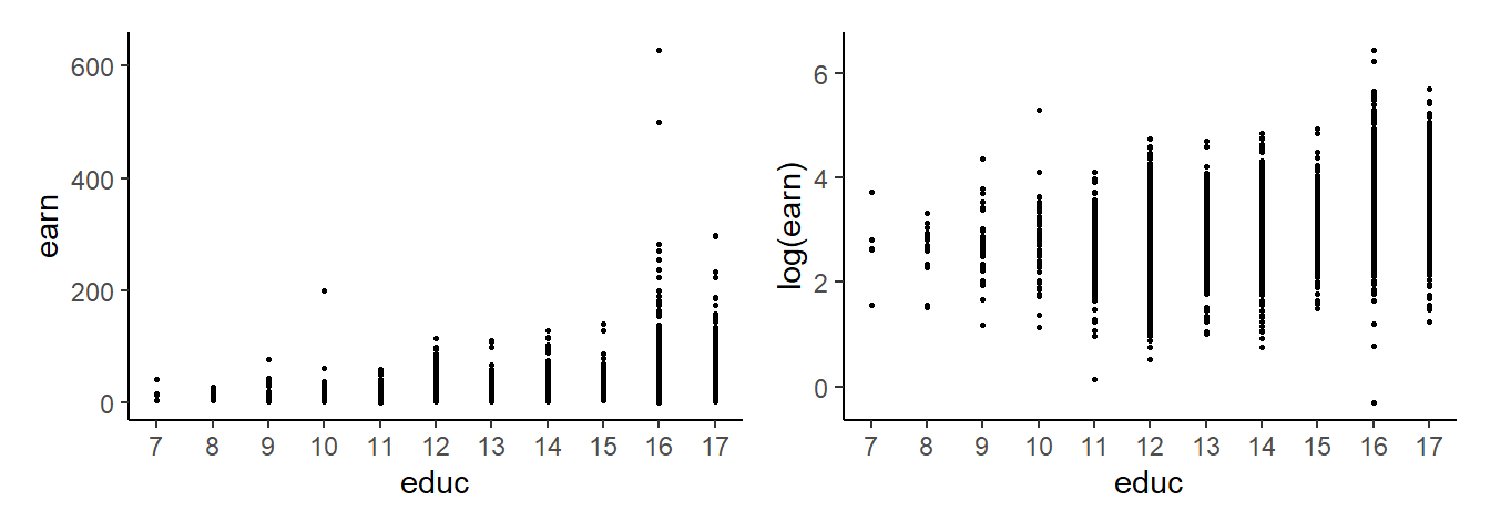

Figure 3.1: Scatterplots of earn and log(earn) against educ.

To be more specific, suppose we are interested in estimating the conditional expectation of ln(earn) given educ, which we assume to be linear, i.e., we want to estimate \[ E(\ln earn \mid educ) = \beta_0 + \beta_1 educ\,. \tag{3.8}\] This means estimating the parameters \(\beta_0\) and \(\beta_1\).

Why do we specify the conditional expectation in log-linear form as in (3.8) rather than the fully linear form \[ E(earn \mid educ) = \beta_0 + \beta_1 educ? \tag{3.9}\] For one thing, we can see from Fig. 3.1 that the log-linear form seems to better describe the data than the fully linear specification. Secondly, (3.9) implies that expected earnings go up by \(\beta_1\) dollars for each additional year of educ, regardless of the level of schooling, i.e., increasing schooling from 7 to 8 leads to the same dollar increase in earnings as increasing schooling from 15 to 16 years. This seems unrealistic. On the other hand, the log-linear form says that expected earnings go up by \(100\beta_1\) percent for each additional year of educ, which seems more realistic.

If we define \[ \epsilon = \ln earn - \beta_0 - \beta_1 educ\,, \tag{3.10}\] then we can write \[ \ln earn = \beta_0 + \beta_1 educ + \epsilon\,. \tag{3.11}\] We will refer to \(\epsilon\) as the noise term, which has the property \[ \begin{aligned} E(\epsilon \mid educ) &= E(\ln earn - \beta_0 - \beta_1 educ \mid educ) \\[1ex] &= E(\ln earn \mid educ) - \beta_0 - \beta_1 educ = 0 \end{aligned} \tag{3.12}\] as long as our specification of the conditional expectation (3.8) is correct. We can write our model of the population as \[ \ln earn = \beta_0 + \beta_1 educ + \epsilon\,,\,E(\epsilon \mid educ) = 0\,. \tag{3.13}\] Equation (3.12) also implies \(E(\epsilon) = 0\).

Let \(\{Y_i, X_i\}_{i=1}^n\) represent your sample, where \(Y_i\) represents \(\ln earn_i\), \(X_i\) represents \(educ_i\), and \(n=4946\). Since your sample is representative of the population, we can write \[ Y_i = \beta_0 + \beta_1 X_i + \epsilon_i\,,\,E(\epsilon_i \mid X_i) = 0\, \text{ for }\, i=1, \dots, n\,. \tag{3.14}\] If your sample is iid, we can extend (3.14) to \[ \begin{aligned} Y_i = \beta_0 + \beta_1 X_i &+ \epsilon_i \\[1ex] E(\epsilon_i \mid X_1, \dots, X_n) &= 0 \\[1ex] E(\epsilon_i\epsilon_j \mid X_1, \dots, X_n) &= 0 \;\text{ for }\; i,j = 1, \dots, n\,,\,\, i\neq j\,. \end{aligned} \tag{3.15}\] This is our simple linear regression model. Given estimators \(\widehat{\beta}_0\) and \(\widehat{\beta}_1\) for \(\beta_0\) and \(\beta_1\), we define the following terms:

Fitted values: \(\widehat{Y}_i = \widehat{\beta}_0 + \widehat{\beta}_1 X_i\),

Residuals: \(\widehat{\epsilon}_i = Y_i - \widehat{Y}_i = Y_i - \widehat{\beta}_0 - \widehat{\beta}_1 X_i\).

for all \(i=1, \dots, n\). Of course, we have \(Y_i = \widehat{Y}_i + \widehat{\epsilon}_i\).

There are a number of ways to obtain estimators \(\widehat{\beta}_0\) and \(\widehat{\beta}_1\). Some approaches lead to the same estimators whereas others produce different estimators. The method of moments approach proceeds as follows: Since your sample is representative of the population and your population satisfies \(E(\epsilon \mid X) = 0\), which implies \[ E(\epsilon) = 0 \;\text{ and }\; E(\epsilon X) = 0\,, \tag{3.16}\] we can choose \(\widehat{\beta}_0\) and \(\widehat{\beta}_1\) so that the sample counterparts of (3.16) also hold, i.e., we choose \(\widehat{\beta}_0\) and \(\widehat{\beta}_1\) such that \[ \begin{aligned} \frac{1}{n}&\sum_{i=1}^n \widehat{\epsilon}_i^{mm} = 0 \\ \frac{1}{n}&\sum_{i=1}^n \widehat{\epsilon}_i^{mm}X_i = 0 \\ \end{aligned} \] where \(\widehat{\epsilon}_i^{mm} = (Y_i - \widehat{\beta}_0^{mm} - \widehat{\beta}_1^{mm}X_i)\).

That is \[ \begin{gathered} \sum_{i=1}^n (Y_i - \widehat{\beta}_0^{mm} - \widehat{\beta}_1^{mm}X_i) = 0 \\ \sum_{i=1}^n (Y_i - \widehat{\beta}_0^{mm} - \widehat{\beta}_1^{mm}X_i)X_i = 0 \end{gathered} \tag{3.17}\] This is a system of two equations which can be solved for the \(\widehat{\beta}_0^{mm}\) and \(\widehat{\beta}_1^{mm}\). We label the estimators with \(mm\) to indicate that they were obtained from the method of moments approach.

Another approach is to say that we want to find \(\widehat{\beta}_0\) and \(\widehat{\beta}_1\) so that the estimated regression line fits the data well in the sense of making the residual sum of squares as small as possible, i.e., choose \[ \widehat{\beta}_0^{ols}, \widehat{\beta}_1^{ols} = \underset{\widehat{\beta}_0\,,\, \widehat{\beta}_1}{\arg \min} \sum\limits_{i=1}^n (Y_i - \hat{\beta}_0 - \hat{\beta}_1 X_i)^2\,. \tag{3.18}\] This is the ordinary least squares (OLS) approach. Elementary optimization theory says that \(\widehat{\beta}_0^{ols}, \widehat{\beta}_1^{ols}\) must satisfy the necessary first-order conditions \[ \begin{aligned} \text{(1) } \;\;\;\;\left.\frac{\partial RSS}{\partial \hat{\beta}_0}\right| _{\hat{\beta}_0^{ols},\,\hat{\beta}_1^{ols}} &= \;\;-2\sum_{i=1}^n(Y_i-\hat{\beta}_0^{ols}-\hat{\beta}_1^{ols}X_i) = 0 \\[1ex] \text{(2) } \;\;\;\; \left.\frac{\partial RSS}{\partial \hat{\beta}_1}\right| _{\hat{\beta}_0^{ols},\,\hat{\beta}_1^{ols}} &= \;\;-2\sum_{i=1}^n(Y_i-\hat{\beta}_0^{ols}-\hat{\beta}_1^{ols}X_i)X_i=0 \end{aligned} \tag{3.19}\] where \(RSS\) refers to the residual sum of squares \(\sum\limits_{i=1}^n (Y_i - \hat{\beta}_0 - \hat{\beta}_1 X_i)^2\). Notice that the conditions (3.19) are the same as the method of moments conditions (3.17) so both approaches lead to the same estimator.

Yet another approach is the least absolute deviation (LAD) approach: \[ \widehat{\beta}_0^{lad}, \widehat{\beta}_1^{lad} = \underset{\widehat{\beta}_0\,,\, \widehat{\beta}_1}{\arg \min} \sum\limits_{i=1}^n \;\lvert\; Y_i - \hat{\beta}_0 - \hat{\beta}_1 X_i \; \rvert\,. \tag{3.20}\] This approach leads to a different set of estimators.

We shall focus on the OLS / MM approach. We will call it the “OLS” approach and label the estimators, fitted values and residuals with an OLS superscript.

3.3.1 OLS Formulas for the Simple Linear Regression Model

Solving (3.19) gives \[ \begin{aligned} \hat{\beta}_0^{ols} &= \overline{Y} - \hat{\beta}_1^{ols}\overline{X} \\[2ex] \hat{\beta}_1^{ols} &= \frac{\sum_{i=1}^n (Y_i-\overline{Y})X_i}{\sum_{i=1}^n(X_i-\overline{X})X_i} = \frac{\sum_{i=1}^n (X_{i} - \overline{X})(Y_i-\overline{Y})}{\sum_{i=1}^n(X_i-\overline{X})^{2}} \end{aligned} \tag{3.21}\] The details are as follows: \[ (1) \;\;\Rightarrow\;\; \sum_{i=1}^n Y_i- n\hat{\beta}_0^{ols}-\hat{\beta}_1^{ols}\sum_{i=1}^n X_i = 0 \;\;\Rightarrow\;\; \overline{Y} - \hat{\beta}_0^{ols}-\hat{\beta}_1^{ols}\overline{X} = 0 \;\;\Rightarrow\;\; \hat{\beta}_0^{ols} = \overline{Y} - \hat{\beta}_1^{ols}\overline{X} \] Substituting \(\hat{\beta}_0^{ols}\) into (2) then gives \[ \begin{aligned} &\sum_{i=1}^n(Y_i-(\overline{Y} - \hat{\beta}_1^{ols}\overline{X})-\hat{\beta}_1^{ols}X_i)X_i=0 \\ &\sum_{i=1}^n[(Y_i-\overline{Y}) - \hat{\beta}_1^{ols}(X_i-\overline{X})]X_i=0 \\ &\sum_{i=1}^n(Y_i-\overline{Y})X_i - \hat{\beta}_1^{ols}\sum_{i=1}^n(X_i-\overline{X})X_i=0 \;\;\;\Rightarrow\;\;\;\hat{\beta}_1^{ols} = \frac{\sum_{i=1}^n(Y_i-\overline{Y})X_i}{\sum_{i=1}^n(X_i-\overline{X})X_i}\,. \end{aligned} \] Since \(\sum_{i=1}^n(Y_i - \overline{Y})X_i = \sum_{i=1}^n(X_i - \overline{X})(Y_i - \overline{Y}) = \sum_{i=1}^n(X_i - \overline{X})Y_i\), we can also write \(\hat{\beta}_1^{ols}\) as \[ \hat{\beta}_1^{ols} = \frac{\sum_{i=1}^n(X_i-\overline{X})(Y_i-\overline{Y})}{\sum_{i=1}^n(X_i-\overline{X})^2} \tag{3.22}\] or even \[ \hat{\beta}_1^{ols} = \frac{\frac{1}{n-1}\sum_{i=1}^n(X_i-\overline{X})(Y_i-\overline{Y})}{\frac{1}{n-1}\sum_{i=1}^n(X_i-\overline{X})^2} = \frac{\text{sample covariance}(X_i, Y_i)}{\text{sample variance}(X_i)}\,. \tag{3.23}\] Ultimately, \(\widehat{\beta}_1^{ols}\) measures the sample covariance between \(X_i\) and \(Y_i\), scaled by the sample variance of \(X_i\).

From (3.23) it should be clear that we need \[ \sum_{i=1}^n(X_i-\overline{X})^2 \neq 0\,, \] i.e., we need the sample variance of \(X_i\) to be greater than zero, in order to get an OLS estimator for \(\beta_1\). This makes sense. The parameter \(\beta_1\) measures how \(Y_i\) varies with \(X_i\) in your data. To make this measurement you must have variation in your regressor \(X_i\).

Notice also that we can write \[ \hat{\beta}_1^{ols} = \frac{\sum_{i=1}^n(X_i-\overline{X})Y_i}{\sum_{i=1}^n(X_i-\overline{X})^2} = \sum_{i=1}^n\left(\frac{(X_i-\overline{X})}{\sum_{i=1}^n(X_i-\overline{X})^2}\right) Y_i = \sum_{i=1}^n w_i Y_i\,. \] where \(w_i = (X_i - \overline{X})/\sum_{i=1}^n(X_i - \overline{X})^2\). Any estimator that can be written as a weighted sum of \(Y_i\) is called a linear estimator.

Once you have \(\widehat{\beta}_1^{ols}\), you can obtain \(\widehat{\beta}_0^{ols}\) from the first equation in (3.21). The estimated model (the sample regression line) is \[ \hat{Y} = \hat{\beta}_0^{ols} + \hat{\beta}_1^{ols} X\,. \tag{3.24}\] The OLS fitted values are: \[ \hat{Y}_i^{ols} = \hat{\beta}_0^{ols} + \hat{\beta}_1^{ols} X_i\,,\,\,i=1,\dots,n\,. \tag{3.25}\] The OLS residuals are \[ \widehat{\epsilon}_i^{ols} = Y_i - \hat{Y}_i^{ols} = Y_i - \hat{\beta}_0^{ols} - \hat{\beta}_1^{ols} X_i\,,\,\, i=1,\dots,n\,. \tag{3.26}\]

3.4 Properties of the OLS Estimators

We shall focus on \(\widehat{\beta}_1\). Similar remarks hold for \(\widehat{\beta}_0\) but the details for \(\widehat{\beta}_0\) are best left for when we discuss the general multiple linear regression case.

3.4.1 Unbiasedness

First rewrite \(\hat{\beta}_1^{ols}\) as \[ \begin{aligned} \hat{\beta}_1^{ols} \;&=\; \frac{\sum_{i=1}^n(X_i-\overline{X})Y_i}{\sum_{i=1}^n(X_i-\overline{X})^2} \\[1ex] \;&=\; \frac{\sum_{i=1}^n(X_i-\overline{X})(\beta_0 + \beta_1 X_i + \epsilon_i)}{\sum_{i=1}^n(X_i-\overline{X})X_i} \\[1ex] &=\; \frac{\beta_0\sum_{i=1}^n(X_i-\overline{X})+ \beta_1 \sum_{i=1}^n(X_i-\overline{X})X_i + \sum_{i=1}^n (X_i-\overline{X})\epsilon_i)}{\sum_{i=1}^n(X_i-\overline{X})X_i} \\[1ex] &=\; \beta_1 + \frac{\sum_{i=1}^n (X_i-\overline{X})\epsilon_i}{\sum_{i=1}^n(X_i-\overline{X})X_i}\,. \end{aligned} \tag{3.27}\] Then \[ E(\hat{\beta}_1^{ols} \mid X_1, \dots, X_n) \;=\; \beta_1 + \frac{\sum_{i=1}^n (X_i-\overline{X})E(\epsilon_i \mid X_1, \dots, X_n)}{\sum_{i=1}^n(X_i-\overline{X})X_i} \;=\; \beta_1\,. \] It follows that \[ E(\hat{\beta}_1^{ols}) = \beta_1\,. \] That is, \(\hat{\beta}_1^{ols}\) is unbiased for \(\beta_1\) . By following the OLS approach, you will not systematically over- or under-estimate \(\beta_1\). Notice, however, that we made use of the assumption \(E(\epsilon_i \mid X_1, \dots, X_n) = 0\) which in turn depends on the assumption that we specified the conditional expectation correctly. There are other reasons that might cause \(E(\epsilon_i \mid X_1, \dots, X_n) = 0\) to fail to hold. We shall come to them in due course.

3.4.2 Consistency

The OLS estimator \(\hat{\beta}_1^{ols}\) is also consistent for \(\beta_1\). We present two rough arguments.

Rough argument 1: \[ \hat{\beta}_1^{ols} = \dfrac{\sum_{i=1}^n(X_i-\overline{X})(Y_i - \overline{Y})}{\sum_{i=1}^n(X_i - \overline{X})^2} = \dfrac{\frac{1}{n}\sum_{i=1}^n(X_i-\overline{X})(Y_i - \overline{Y})}{\frac{1}{n}\sum_{i=1}^n(X_i - \overline{X})^2}\,. \tag{3.28}\] Appealing to LLN:

Numerator converges in probability to population \(\mathit{Cov}(X, Y)\).
Denominator converges in probability to population \(\mathit{Var}(X)\).

\[ \hat{\beta}_1^{ols} = \dfrac{\frac{1}{n}\sum_{i=1}^n(X_i-\overline{X})(Y_i - \overline{Y})}{\frac{1}{n}\sum_{i=1}^n(X_i - \overline{X})^2} \overset{p}\longrightarrow \frac{\mathit{Cov}(X,Y)}{\mathit{Var}(X)} = \beta_1\,. \tag{3.29}\] Rough argument 2: \[ \hat{\beta}_1^{ols} = \beta_1 + \dfrac{\sum_{i=1}^n(X_i-\overline{X})\epsilon_i}{\sum_{i=1}^n(X_i - \overline{X})^2} = \beta_1 + \dfrac{\frac{1}{n}\sum_{i=1}^n(X_i-\overline{X})\epsilon_i}{\frac{1}{n}\sum_{i=1}^n(X_i - \overline{X})^2}\,. \tag{3.30}\]

Numerator in second term converges in probability to population \(\mathit{Cov}(X,\epsilon)\).
Denominator in second term converges in probability to population \(\mathit{Var}(X)\).

If population \(\mathit{Cov}(X,\epsilon) = 0\) and population \(\mathit{Var}(X) \neq 0\), then \[ \hat{\beta}_1^{ols} \;\;=\;\; \beta_1 + \dfrac{\frac{1}{n}\sum_{i=1}^n(X_i-\overline{X})\epsilon_i}{\frac{1}{n}\sum_{i=1}^n(X_i - \overline{X})^2} \;\;\overset{p}\longrightarrow\;\; \beta_1 + \frac{\mathit{Cov}(X,\epsilon)}{\mathit{Var}(X)} = \beta_1\,. \tag{3.31}\]

3.4.3 Standard Errors

Standard errors should be calculated for all estimators. For \(\widehat{\beta}_1^{ols}\), we have \[ \begin{aligned} \hat{\beta}_1^{ols} &= \beta_1 + \dfrac{\sum_{i=1}^n(X_i-\overline{X})\epsilon_i}{\sum_{i=1}^n(X_i - \overline{X})^2} \\[1ex] \mathit{Var}(\hat{\beta}_1^{ols} \mid X_1, \dots, X_n) &= \dfrac{\sum_{i=1}^n(X_i-\overline{X})^2\mathit{Var}(\epsilon_i \mid X_1, \dots, X_n)}{(\sum_{i=1}^n(X_i - \overline{X})^2)^2} \end{aligned} \tag{3.32}\] If we are willing to assume, in addition to all the assumptions we have made so far, that \[ \mathit{Var}(\epsilon_i \mid X_1, \dots, X_n) = \sigma^2 \tag{3.33}\] then (3.32) simplifies to \[ \begin{aligned} \mathit{Var}(\hat{\beta}_1^{ols} \mid X_1, \dots, X_n) &= \dfrac {\sum_{i=1}^n(X_i-\overline{X})^2\overbrace{\mathit{Var}(\epsilon_i \mid X_1, \dots, X_n)}^{\sigma^2}} {(\sum_{i=1}^n(X_i - \overline{X})^2)^2} \\[1ex] &= \dfrac {\sigma^2\sum_{i=1}^n(X_i-\overline{X})^2} {(\sum_{i=1}^n(X_i - \overline{X})^2)^2} \\[1ex] &= \dfrac{\sigma^2}{\sum_{i=1}^n(X_i - \overline{X})^2}\,. \end{aligned} \tag{3.34}\] In order to get a numerical estimate for the variance, we have to get an estimate for \(\sigma^2\). Nonetheless, (3.34) is informative. It says that the OLS estimator \(\widehat{\beta}_1\) has a smaller variance if (i) \(\sigma^2\) is small (the data is less noisy), (ii) \(n\) is larger (since the denominator is a sum of \(n\) non-negative terms) and (iii) if there is more variation in your \(X_i\) sample.

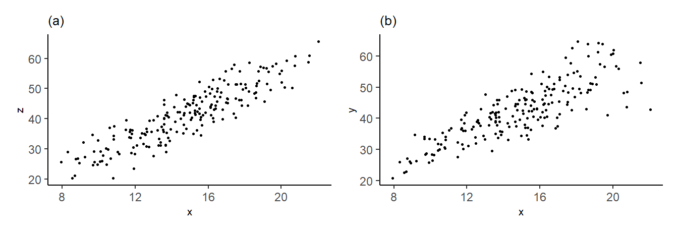
The assumption (3.33) is called homoskedasticity. It will hold if \(\mathit{Var}(\epsilon \mid X)\) is constant in population and you have a representative iid sample from the population. It says that the “noisiness” of the data does not depend on any of the \(X\) observations. If \(\mathit{Var}(\epsilon_i \mid X_1, \dots, X_n)\) is not constant, then we say there is heteroskedasticity. Fig. 3.2 shows data from the data set heterosk.csv. In (a), for a regression of \(Z\) on \(X\), the error terms appear homoskedastic whereas in (b), for a regression of \(Y\) on \(X\), the error terms appear to be heteroskedastic, in particular, the variance appears to be increasing in \(X\).

Figure 3.2: (a) Homoskedastic errors, (b) Heteroskedastic errors,

The formula (3.34) is valid only in the homoskedasticity case. In that case, it can be shown that an unbiased estimator for \(\sigma^2\) is \[ \widehat{\sigma^2} = \frac{1}{n-2}\sum_{i=1}^n \widehat{\epsilon}_{i,ols}^2\,. \] We define the standard error of \(\widehat{\beta}_1\) as \[ \text{s.e.}(\widehat{\beta}_1) = \sqrt{\frac{\widehat{\sigma^2}}{\sum_{i=1}^n(X_i - \overline{X})^2}}\,\,. \] Furthermore, if \(\epsilon_i \sim \text{Normal}(0, \sigma^2)\), we have \[ \text{t-stat} = \frac{\widehat{\beta}_1^{ols}-\beta_1}{\text{s.e.}(\widehat{\beta}_1)} \;\;\sim\;\; \text{t}(n-2)\,. \] If not, we can appeal to the asymptotic result \[ t = \frac{\widehat{\beta}_1^{ols}-\beta_1}{\text{s.e.}(\widehat{\beta}_1)} \;\;\overset{a}{\sim}\;\; \text{Normal}(0,1)\,. \] The t-stat can be used to test hypotheses on \(\beta_1\).

Example 3.2 For our returns to education example, using data in earn2019.csv, we have

slr <- function(y, x){
  n <- length(y)
  ybar <- mean(y)
  xbar <- mean(x)
  beta1hat <- sum((x-xbar)*y)/sum((x-xbar)*x)
  beta0hat <- ybar - beta1hat*xbar
  yhat <- beta0hat + beta1hat*x
  ehat <- y - yhat
  rss <- sum(ehat^2)
  beta1hat_se <- sqrt((rss/(n-2))/sum((x-xbar)^2))
  beta1hat_t <- beta1hat / beta1hat_se
  cat("beta0hat:", round(beta0hat,3), "\n")
  cat("beta1hat:", round(beta1hat,3), 
      "  s.e.:", round(beta1hat_se,3), 
      "  t-stat:", round(beta1hat_t,3),
      "  p-val:", round(2*pt(-abs(beta1hat_t), n-2),3))
  results <- list(beta0hat=beta0hat, beta1hat=beta1hat, 
                  beta1hat_se=beta1hat_se, ehat=ehat, yhat=yhat)
}

cat("Regression of ln earn on educ, with intercept\n\n")
mdl1 <- slr(y=log(dat1$earn), x=dat1$educ)

Regression of ln earn on educ, with intercept

beta0hat: 1.32 
beta1hat: 0.128   s.e.: 0.004   t-stat: 32.17   p-val: 0

We left out the standard error for \(\widehat{\beta}_0\) since we haven’t yet developed the formula for it (we will do so in a later chapter). The t-statistic for \(\widehat{\beta}_1\) is calculated as \(\widehat{\beta}_1 / \text{s.e.}(\widehat{\beta}_1)\) and is meant for testing the hypothesis \(\beta_1 = 0\). The associate p-value for this test is also given.

Instead of writing your own code, you can use R’s built-in lm() function to estimate the regression:

mdl1a <- lm(log(earn)~educ, dat1) 
cat("Dependent variable: ", as.character(formula(mdl1a))[2], "\n")
mdl1a %>% summary() %>% coef()
cat("n =", nobs(mdl1a))

Dependent variable:  log(earn) 
             Estimate  Std. Error  t value      Pr(>|t|)
(Intercept) 1.3199894 0.057541299 22.93986 9.401431e-111
educ        0.1279965 0.003978753 32.17000 2.442343e-206
n = 4946

The data, the sample regression line and the histogram of the residuals are shown in Fig. 3.3.

regdat <- data.frame(educ=dat1$educ, earn=dat1$earn, fitted=mdl1$yhat, resid=mdl1$ehat)
p1 <- ggplot(data=regdat) + 
        geom_point(aes(y=log(earn), x=educ), size=0.5) + 
        geom_point(aes(y=fitted, x=educ), size=1.5, color='blue') + 
        geom_abline(intercept=mdl1$beta0hat, slope=mdl1$beta1hat, color='red') +
        theme_classic()
p2 <- ggplot(regdat, aes(x = resid)) + 
  geom_histogram(aes(y = after_stat(density)), fill = "lightblue", color="black", bins=30) + 
  xlab("residuals") + theme_bw()
p1 | p2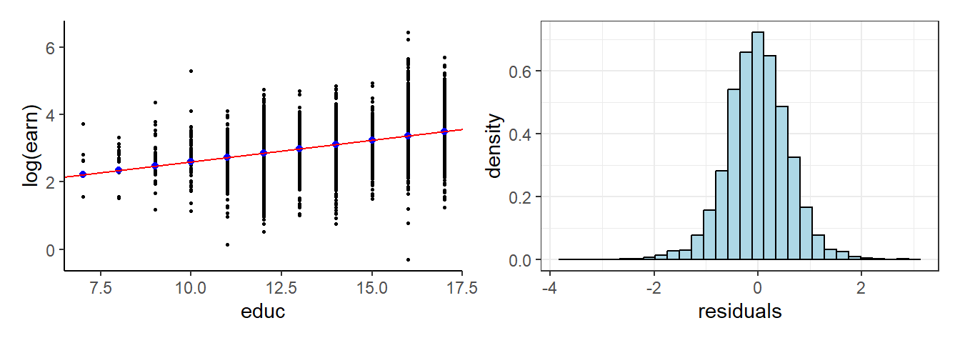

Figure 3.3: Regression of ln(earn) on educ.

What if you are unsure if your errors are homoskedastic? When deriving the variance of \(\widehat{\beta}_1\), we obtained (3.32), repeated below: \[ \mathit{Var}(\hat{\beta}_1^{ols} \mid X_1, \dots, X_n) = \dfrac{\sum_{i=1}^n(X_i-\overline{X})^2\mathit{Var}(\epsilon_i \mid X_1, \dots, X_n)}{(\sum_{i=1}^n(X_i - \overline{X})^2)^2}\,. \] If \(\mathit{Var}(\epsilon_i \mid X_1, \dots, X_n)\) is not a constant, we cannot bring it out of the summation in the numerator, as we did in the derivation of the variance formula in the homoskedasticity case. Without specifying \(\mathit{Var}(\epsilon_i \mid X_1, \dots, X_n)\) any further, we cannot proceed with the derivation. However, it can be shown that under quite general conditions, replacing \(\mathit{Var}(\epsilon_i \mid X_1, \dots, X_n)\) with the squared residuals produces a consistent estimator for the variance of \(\widehat{\beta}_1\) even under heteroskedasticity, i.e., \[ \widehat{\mathit{Var}}_{HC}(\hat\beta_1^{ols}) \;=\; \frac{\sum_{i=1}^n (X_i-\overline{X})^2\,\widehat\epsilon_{i,ols}^2}{\left(\sum_{i=1}^n (X_i-\overline{X})^2\right)^2} \;\;\overset{p}\longrightarrow \;\; \mathit{Var}(\hat\beta_1^{ols})\,. \] This variance estimator is called the heteroskedasticity-robust / heteroskedasticy-consistent / White standard errors. Consistency holds despite the fact that \(E(\widehat\epsilon_{i,ols}^2)\) is in general a biased and inconsistent estimator for \(\mathit{Var}(\epsilon_i)\). Furthermore, \(\widehat{\mathit{Var}}_{HC}(\hat\beta_1^{ols})\) remains consistent even under homoskedasticity. Some researchers use this as their default variance estimator.

slr_hc0 <- function(y, x){
  n <- length(y)
  ybar <- mean(y)
  xbar <- mean(x)
  beta1hat <- sum((x-xbar)*y)/sum((x-xbar)*x)
  beta0hat <- ybar - beta1hat*xbar
  yhat <- beta0hat + beta1hat*x
  ehat <- y - yhat
  hc0 <- sum((x-xbar)^2*ehat^2)/sum((x-xbar)^2)^2
  beta1hat_se <- sqrt(hc0)
  beta1hat_t <- beta1hat / beta1hat_se
  cat("beta0hat:", round(beta0hat,3), "\n")
  cat("beta1hat:", round(beta1hat,3), 
      "  s.e. (het. robust):", round(beta1hat_se,4), 
      "  t-stat:", round(beta1hat_t,3),
      "  p-val:", round(2*pt(-abs(beta1hat_t), n-2),4))
  results <- list(beta0hat=beta0hat, beta1hat=beta1hat, 
                  beta1hat_se=beta1hat_se, ehat=ehat, yhat=yhat)
}
mdl2 <- slr_hc0(y=log(dat1$earn), x=dat1$educ)

beta0hat: 1.32 
beta1hat: 0.128   s.e. (het. robust): 0.0041   t-stat: 31.584   p-val: 0

Alternatively, you can use the coeftest() function from the lmtest package together with the vcovHC function from the sandwich package in the following way. The reason for the sandwich package name will be explained in a later chapter.

library(lmtest)     # lmtest::coeftest to calculate t-test
library(sandwich)   # using robust s.e. calculated with sandwich::vcovHC
coeftest(mdl1a, vcov=vcovHC, type="HC0")  # Robust standard errors 
#NB: mdl1a was estimated earlier using the lm() function


t test of coefficients:

             Estimate Std. Error t value  Pr(>|t|)    
(Intercept) 1.3199894  0.0581594  22.696 < 2.2e-16 ***
educ        0.1279965  0.0040525  31.584 < 2.2e-16 ***
---
Signif. codes:  0 '***' 0.001 '**' 0.01 '*' 0.05 '.' 0.1 ' ' 1

The OLS coefficient estimates are the same, of course. We are only re-calculating the standard errors. As it turns out, the standard errors are very similar, suggesting that heteroskedasticity is not much of an issue here.

3.4.4 Using the Estimated Regression Model

3.4.4.1 Prediction

We can use our estimated model \[ \begin{aligned} \widehat{\ln earn} &= 1.32 \;\;\;\;+\;\;\;\; 0.128\; educ \\ &\;(0.0582) \quad\quad(0.0041) \end{aligned} \] for predictive purposes. Imagine going back to the population and sampling one more individual with, say, 12 years of educ. What is the model’s prediction for this individual’s ln(earn)? The model predicts that this individual’s average hourly earnings ln(earn) to be

cat("Predicted ln ave. hr. earn for individual with 12 years educ is ")
cat(round(mdl1$beta0hat + mdl1$beta1hat*12,2), "\"log-dollars\"")

Predicted ln ave. hr. earn for individual with 12 years educ is 2.86 "log-dollars"

Of course, the scatterplot in Fig. 3.1(b) suggests that the potential error of this prediction might be quite high, the reason being that there are many factors that affect earnings, and these have not been accounted for in the model. Since the parameter estimates are unbiased, we can expect the prediction to also be unbiased (to be correct on average) but the prediction standard error (which we will consider later in the course) would also be quite high.

The model gives predictions for ln earn. To convert this to earn you can take exponentials. In view of the comments at the end of the previous chapter, you might view this as a “conditional median prediction” rather than a “conditional expectation prediction”.

cat("Predicted ave. hr. earn for individual with 12 years educ is ")
cat(round(exp(mdl1$beta0hat + mdl1$beta1hat*12),2), "dollars (cond. median pred.).")

Predicted ave. hr. earn for individual with 12 years educ is 17.39 dollars (cond. median pred.).

3.4.4.2 Measuring direct causal effects?

The model that we just estimated also predicts that an individual with one more year in educ will have 12.8% higher average hourly earnings. Can we take this to mean that every additional year of schooling directly “causes” average hourly earnings to go up by 12.8%? One has to be very careful when interpreting regression results from a causal perspective. The problem again is that there are many factors that affect earnings, and your regression is taking into account only the effect of educ. All of the other factors’ influence on ln earn may end up being attributed to educ.

For instance, suppose there are two factors \(X\) and \(Z\) that affect \(Y\), and that the conditional expectation of \(Y\) given \(X\), and of \(Y\) given \(X\) and \(Z\) are \[ \begin{aligned} E(Y \mid X) &= \alpha_0 + \alpha_1 X\,, \\[1ex] E(Y \mid X, Z) &= \beta_0 + \beta_1 X + \beta_2 Z\,. \end{aligned} \tag{3.35}\] If your intention is to capture the direct effect of \(X\) on \(Y\), then you would want to estimate \(\beta_1\), not \(\alpha_1\). The parameter \(\beta_1\) tells you how the expected value of \(Y\) differs with \(X\) for two individuals in your population with the same \(Z\): \[ E(Y | X=x_0+1, Z=z_0) - E(Y | X=x_0, Z=z_0) = \beta_1\,. \] Since \(Z\) is unchanged, the difference in the expected value of \(Y\) must be due the difference in \(X\). We say that \(\beta_1\) measures the effect of \(X\) on \(Y\) controlling for \(Z\).

A simple linear regression of \(Y\) on \(X\), however, will give you an unbiased estimator for \(\alpha_1\), not \(\beta_1\), and it is straightforward to show that if \(\beta_2 \neq 0\) and \(\mathit{Cov}(X, Z) \neq 0\), then \(\alpha_1 \neq \beta_1\). We have \[ \begin{aligned} E_{Y \mid X}(Y \mid X) &= E_{Z \mid X} (E_{Y \mid X, Z}(Y \mid X, Z)) \\[1ex] &= E_{Z \mid X} (\beta_0 + \beta_1 X + \beta_2 Z) \\[1ex] &= \beta_0 + \beta_1 X + \beta_2 E_{Z \mid X}(Z \mid X)\,. \end{aligned} \tag{3.36}\] Suppose that \(E_{Z \mid X}(Z \mid X) = \delta_0 + \delta_1 X\). Then (3.36) becomes \[ \begin{aligned} E(Y \mid X) &= \beta_0 + \beta_1 X + \beta_2(\delta_0 + \delta_1 X) \\[1ex] &= (\beta_0 + \beta_2 \delta_0) + (\beta_1 + \beta_2\delta_1)X. \end{aligned} \tag{3.37}\] From Exercise 3.7, we know that if \(E_{Z \mid X}(Z \mid X) = \delta_0 + \delta_1 X\), then \[ \delta_0 = E(Z) - \delta_1 E(X)\;\text{ and } \; \delta_1 = \frac{\mathit{Cov}(X, Z)}{\mathit{Var}(X)}\,. \tag{3.38}\] Substituting these into (3.37) gives \[ E(Y \mid X) = (\beta_0 + \beta_2 \delta_0) + \left(\beta_1 + \beta_2\frac{\mathit{Cov}(X, Z)}{\mathit{Var}(Z)}\right) X\,. \tag{3.39}\] Comparing (3.39) with \(E(Y \mid X) = \alpha_0 + \alpha_1X\), we see that \[ \alpha_1 = \beta_1 + \beta_2\frac{\mathit{Cov}(X, Z)}{\mathit{Var}(Z)} \tag{3.40}\] so \(\alpha_1 \neq \beta_1\) unless \(\beta_2 = 0\) or \(\mathit{Cov}(X, Z) = 0\). A simple linear regression of \(Y\) on \(X\) gives you an unbiased estimator for \(\alpha_1\), but a biased estimator for \(\beta_1\).

Here is another way of looking at this issue. Suppose we have \[ E(Y \mid X, Z) = \beta_0 + \beta_1 X + \beta_2 Z \] and define \(u = Y - \beta_0 - \beta_1X - \beta_2 Z\). Then we can write \[ Y = \beta_0 + \beta_1 X + \beta_2 Z + u\,,\,\,E(u \mid X, Z) = 0\,. \tag{3.41}\] Suppose \(X\) and \(Z\) are correlated. Then if we write \[ Y = \beta_0 + \beta_1 X + \epsilon \tag{3.42}\] where the \(\beta_0\) and \(\beta_1\) in (3.42) are the same as the \(\beta_0\) and \(\beta_1\) in (3.41), then \[ \epsilon = \beta_2 Z + u\,. \] If \(X\) and \(Z\) are correlated, then \(\epsilon\) and \(X\) must be correlated, so we no longer have \(E(\epsilon \mid X) = 0\). This causes the OLS estimator for \(\beta_1\) in the simple linear regression of \(Y\) on \(X\) to be biased for \(\beta_1\).

Example 3.3 The file multireg_eg.csv contains observations on variables \(X\), \(Y\) and \(Z\). The variable \(Z\) takes on integer values 1 to 5 only. Fig. 3.4(a) shows a scatterplot of \(Y\) against \(X\). Fig. 3.4(b) shows the same scatterplot, but this time the value of \(Z\) corresponding to each (\(X\),\(Y\)) pair is indicated.

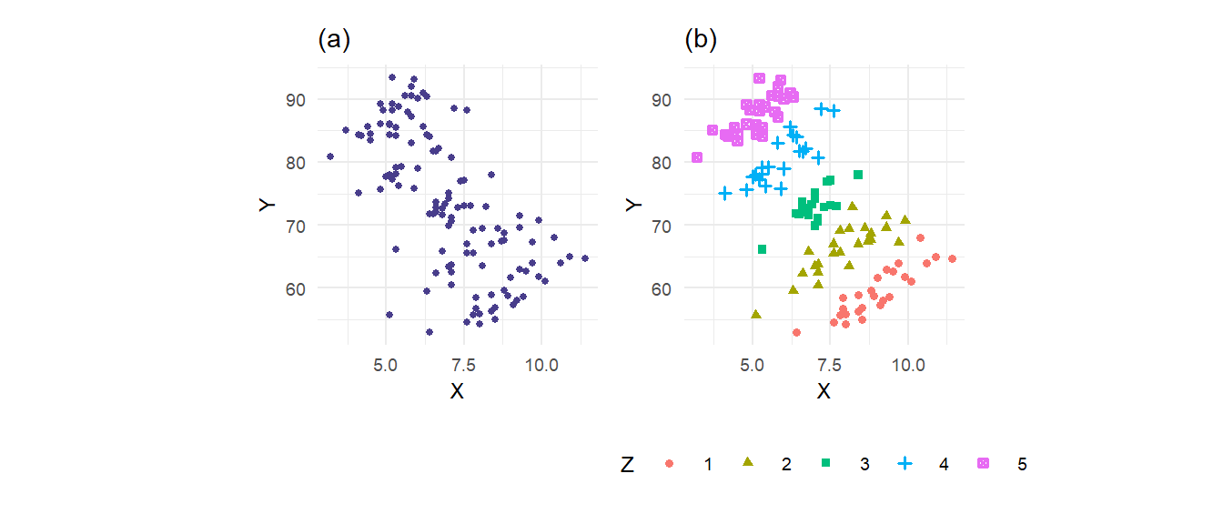
Figure 3.4: Illustrating confounding factors.

The scatterplot in Fig. 3.4(a) shows a strong negative relationship between \(X\) and \(Y\). Yet Fig. 3.4(b) shows that for any fixed level of \(Z\), the effect of \(X\) on \(Y\) is actually positive. What is going on here is that the variable \(Z\), which is negatively correlated with \(X\) (the observations drift left as \(Z\) goes from 1 to 5), also affects \(Y\) positively, for any fixed \(X\). Therefore an increase in \(X\), which tends to increase \(Y\), also tends to be accompanied by a fall in \(Z\), which leads to a fall in \(Y\). The latter effect is strong enough that higher values of \(X\) become associated with lower values of \(Y\). We refer to \(Z\) as a confounding variable.

Imagine, for instance, that \(Y\) represents final exam scores in a certain course, \(Z\) is the background preparedness of the students ranging from very poor (1) to excellent (5), and \(X\) is study hours per week. Given any level of preparedness, studying clearly increases test scores. Background preparedness is also positively correlated with final exam scores. Because students who have strong background preparedness spend less time studying for the course (they probably allocate study time to the courses that they are less prepared for), when we look at test scores vs study time, it will appear that studying reduces test scores.

In this example, clearly \(\alpha_1\) is negative in \[ E(Y \mid X) = \alpha_0 + \alpha_1 X \\\ \] and a simple linear regression of \(Y\) on \(X\) produces

lm(Y~X, data=df) %>% summary() %>% coef()

             Estimate Std. Error  t value     Pr(>|t|)
(Intercept) 102.86406  3.2199095 31.94626 6.373574e-60
X            -4.23213  0.4474755 -9.45779 3.857133e-16

The separate effects of \(X\) and \(Z\) on \(Y\) are captured in the conditional expectation \[ E(Y \mid X, Z) = \beta_0 + \beta_1 X + \beta_2 Z\,. \] In this example, \(\beta_1\) is positive since for any fixed \(Z\), the relationship between \(Y\) and \(X\) is positive. How might we get estimates of these separate effects? Looking ahead to the next chapter, we see that a multiple linear regression of \(Y\) on \(X\) and \(Z\) manages to disentangle the effects

lm(Y~X+Z, data=df) %>% summary() %>% coef()

             Estimate Std. Error  t value     Pr(>|t|)
(Intercept) 21.188337  2.0816539 10.17861 8.212834e-18
X            3.114465  0.2054364 15.16024 2.219609e-29
Z           10.109717  0.2379845 42.48057 5.955647e-73

We shall explore multiple linear regression in more detail in the next chapter — why it works in disentangling causal effects, when it works well, when it does not, and what are the trade-offs.

3.5 Chapter 3 Exercise B

Exercise 3.10 Let \(\widehat{\beta}_0^{ols}\) and \(\widehat{\beta}_1^{ols}\) be the OLS estimators for \(\beta_0\) and \(\beta_1\) in the linear regression model \[ Y_i = \beta_0 + \beta_1 X_i + \epsilon_i \] estimated on the sample \(\{X_i, Y_i\}_{i=1}^n\). Let \(\widehat{\epsilon}_i^{ols}\) and \(\widehat{Y}_i^{ols}\), \(i=1, \dots, n\), be the OLS residuals and fitted values.

Explain why the OLS residuals have sample mean equal to zero, and that the OLS residuals and regressors \(X_i\) are orthogonal (meaning that \(\sum_{i=1}^n X_i \widehat{\epsilon}_i^{ols} = 0\)).
Show that \(\overline{Y} = \overline{\widehat{Y}}\) where \(\overline{\widehat{Y}}\) is the sample mean of the fitted values.
Explain why the OLS residuals and regressors \(X_i\) are uncorrelated.
Explain why the OLS residuals and OLS fitted values are uncorrelated.
Show that the estimated regression line always passes through the point \((\overline{X}, \overline{Y})\).
When will \(\widehat{\beta}_1^{ols} = 0\)? What will \(\widehat{\beta}_0^{ols}\) be in this case?
If \(\overline{X} = 0\), show that \(\widehat{\beta}_1^{ols}\) reduces to \[ \widehat{\beta}_1^{ols} = \dfrac{\sum_{i=1}^n X_iY_i}{\sum_{i=1}^n X_i^2}\,. \] What will \(\widehat{\beta}_0^{ols}\) be in this case?

Exercise 3.11 The simple linear regression without intercept is the model \[ Y_i = \beta_1 X_i + \epsilon_i\,i = 1, \dots, n\,. \] (a) Derive the OLS estimator for \(\beta_1\).

(b) Explain why the OLS residuals now need not have sample mean equal to zero.

(d) For OLS estimation of the linear regression model with intercept, we required that there be some variation in your regressors, i.e., we cannot have \(X_1 = \dots = X_n = c\) for some fixed value \(c\). Explain why OLS estimation of the linear regression model without intercept is still possible even if there is no variation in \(X_i\).

Exercise 3.12 For the simple linear regression with intercept, estimated by OLS on the dataset \(\{X_i, Y_i\}_{i=1}^n\), define the OLS fitted values \(\{\widehat{Y}_{i}\}_{i=1}^n\) and residuals \(\{\widehat{\epsilon}_{i}\}_{i=1}^n\) in the usual way, so that \[ Y_i = \widehat{Y}_{i} + \widehat{\epsilon}_{i}\,,\,\,i=1, \dots, n\,. \] To simplify notation, we drop the “ols” subscripts from the residuals and fitted values.

(a) Show that \(\sum_{i=1}^n Y_i^2 = \sum_{i=1}^n\widehat{Y}_{i}^2 + \sum_{i=1}^n\widehat{\epsilon}_{i}^2\).

(b) Show that \[ \underbrace{\sum_{i=1}^n (Y_i - \overline{Y})^2}_{TSS} \;=\; \underbrace{\sum_{i=1}^n (\widehat{Y}_{i} - \overline{\widehat{Y}})^2}_{FSS} \;+\; \underbrace{\sum_{i=1}^n \widehat{\epsilon}_{i}^2}_{RSS}\,. \tag{3.43}\] This equation can be described as “Total Sum of Squares = Fitted Sum of Squares + Residual Sum of Squares”, or \(TSS = FSS + RSS\).¹ Dividing (3.43) throughout by \(n-1\), the equation can also be described as a variance decomposition, specifically: \[ \text{sample var.}(Y_i) = \text{sample var.}(\widehat{Y}_{i}) + \text{sample var.}(\widehat{\epsilon}_{i}) \tag{3.44}\]

(c) The \(R^2\) is defined as \[ R^2 = 1 - \frac{RSS}{TSS}\,. \] It is used as a measure of goodness-of-fit, since \(RSS=0\) when you have a perfect fit. Where you don’t have a perfect fit, \(RSS > 0\) and therefore \(R^2 < 1\).

When will \(R^2 = 0\)? Can \(R^2\) fall below zero?
What is \(R^2\) for the case where \(Y_1 = \dots = Y_n = c\) for some constant \(c\)?

3.6 Appendix: The Bivariate Normal Distribution

Two random variables \(X\) and \(Y\) have the bivariate normal distribution if their joint pdf have the form \[ f_{X,Y}(x,y) = \frac{1}{2\pi\sigma_x\sigma_y\sqrt{1-\rho_{xy}^2}} \exp\left\{ -\frac{1}{2}\frac{\widetilde{x}^2 - 2\rho_{xy}\widetilde{x} \widetilde{y} + \widetilde{y}^2} {1-\rho_{xy}^2} \right\} \tag{3.45}\] where \(\widetilde{x}=\dfrac{x-\mu_x}{\sigma_x}\) and \(\widetilde{y}=\dfrac{y-\mu_y}{\sigma_y}\). The bivariate normal distribution has five parameters, with the following interpretation:

\(\mu_x\) : unconditional mean of \(X\),
\(\mu_y\) : unconditional mean of \(Y\),
\(\sigma_x^2\) : unconditional variance of \(X\),
\(\sigma_y^2\) : unconditional variance of \(Y\), and
\(\rho_{xy}\) : correlation coefficient of \(X\) and \(Y\), i.e., \(\rho_{xy} = \dfrac{\sigma_{xy}}{\sigma_x\sigma_y}\) where \(\sigma_{xy} = \mathit{Cov}(X,Y)\).

We write \[ (X,Y) \sim \mathrm{Normal}_2(\mu_x, \mu_y, \sigma_x^2, \sigma_y^2, \rho_{xy})\,. \]

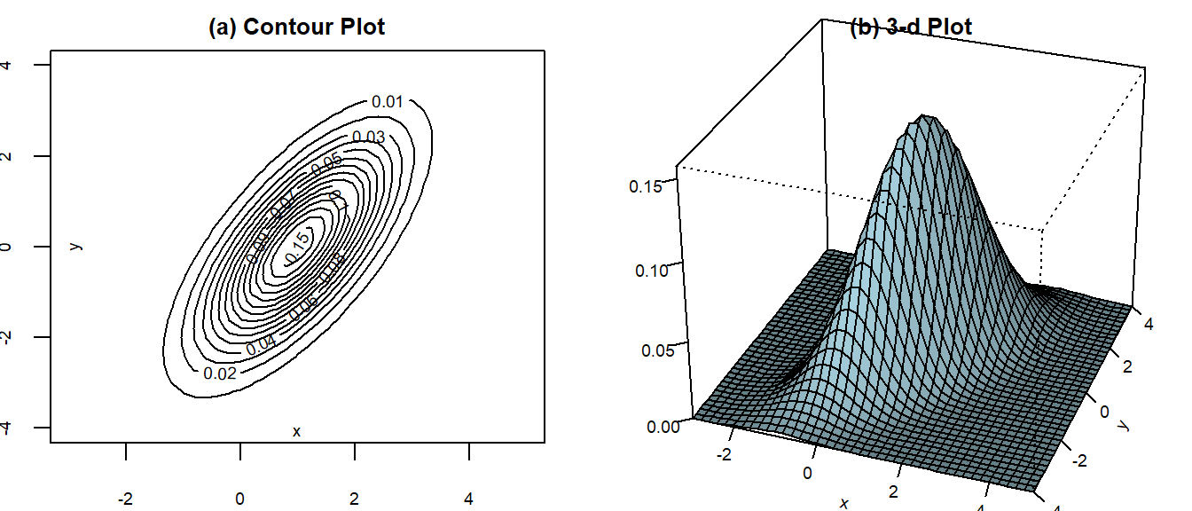
Contour plots are helpful for visualizing bivariate normal distributions. We show the contour plots of a bivariate normal distribution with \[ (\mu_x, \mu_y, \sigma_x^2, \sigma_y^2, \rho_{xy}) = (1, 0, 1, 2, 0.9). \] in Fig. 3.5(a). Alternatively, one can look at the 3D plot of the bivariate pdf in Fig. 3.5(b).

Figure 3.5: Bivariate normal distribution (parameter values given in text).

The marginal and conditional distributions of a bivariate normal random variables are also normal. To see this, we “complete the square” on \(\widetilde{x}^2 - 2\rho_{xy}\widetilde{x} \widetilde{y} + \widetilde{y}^2\) to get \[ \begin{aligned} \widetilde{x}^2 - 2\rho_{xy}\widetilde{x} \widetilde{y} + \widetilde{y}^2 & = (\widetilde{x} - \rho_{xy} \widetilde{y})^2 + (1 - \rho_{xy}^2) \widetilde{y}^2 \\ & = \left[\frac{x - \mu_x}{\sigma_x} - \frac{\sigma_{xy}}{\sigma_x\sigma_y}\frac{y-\mu_y}{\sigma_y} \right]^2 + (1 - \rho_{xy}^2) \left( \frac{y-\mu_y}{\sigma_y} \right)^2 \\ & = \frac{1}{\sigma_x^2}\left[x - \mu_x - \frac{\sigma_{xy}}{\sigma_y^2}(y-\mu_y) \right]^2 + (1 - \rho_{xy}^2) \left( \frac{y-\mu_y}{\sigma_y} \right)^2 \\ & = \frac{1}{\sigma_x^2}\left[x - (\alpha + \beta y) \right]^2 + (1 - \rho_{xy}^2) \left( \frac{y-\mu_y}{\sigma_y} \right)^2 \end{aligned} \]

where \(\alpha = \mu_x - \beta \mu_y\) and \(\beta = \dfrac{\sigma_{xy}^2}{\sigma_y^2}\). Then the pdf can be written as \[ \begin{aligned} &f_{X,Y}(x,y) \\ &= \frac{1}{2\pi\sigma_x\sigma_y\sqrt{1-\rho_{xy}^2}} \exp\left\{-\frac{1}{2} \frac{1}{1-\rho_{xy}^2}(\widetilde{x}^2 - 2\rho_{xy}\widetilde{x} \widetilde{y} + \widetilde{y}^2) \right\} \\ &= \frac{1}{2\pi\sigma_x\sigma_y\sqrt{1-\rho_{xy}^2}} \times \exp\left\{-\frac{1}{2} \frac{1}{1-\rho_{xy}^2} \left[ \frac{1}{\sigma_x^2}\left[x - (\alpha + \beta y) \right]^2 + (1 - \rho_{xy}^2) \left( \frac{y-\mu_y}{\sigma_y} \right)^2 \right] \right\} \\ &=\underbrace{ \frac{1}{\sqrt{2\pi}\sqrt{\sigma_x^2(1-\rho_{xy}^2)}} \exp\left\{-\frac{1}{2} \frac{\left[x - (\alpha + \beta y) \right]^2}{\sigma_x^2(1-\rho_{xy}^2)} \right\} }_{A} \times \underbrace{ \frac{1}{\sqrt{2\pi}\sigma_y} \exp\left\{ -\frac{1}{2} \left( \frac{y-\mu_y}{\sigma_y} \right)^2 \right\} }_{B} \end{aligned} \] If we compare expressions \(A\) and \(B\) with the expression for the normal pdf, we see that \(B\) is a normal pdf \(f_Y(y)\) with mean \(\mu_y\) and variance \(\sigma_y\), and if we take \(y\) as fixed, then \(A\) is a (conditional) normal pdf \(f_{X \mid Y}(x \mid y)\) with mean \(\alpha + \beta y\) and variance \(\sigma_x^2 - \sigma_{xy}^2/\sigma_y^2\). That is, if \(X\) and \(Y\) have the bivariate normal distribution (3.45), then

the marginal distribution of \(Y\) is \(\mathrm{Normal}(\mu_y, \sigma_y^2)\),

the conditional distribution of \(X\) given \(Y\) is \(\mathrm{Normal}(\mu_{x \mid y}, \sigma_{x \mid y}^2)\) where

\[ \mu_{x \mid y} = \mu_x + \frac{\sigma_{xy}}{\sigma_y^2}(y-\mu_y)\;\; \text{ and } \;\; \sigma_{x \mid y}^2 = \sigma_x^2 - \dfrac{\sigma_{xy}^2}{\sigma_y^2}. \]

Notice that the condition mean of \(X\) given \(Y\) is linear in \(Y\). It can be written as \[ \mu_{x \mid y} = \alpha_x + \beta_x y \] where \(\alpha_x = \mu_x - \beta_x \mu_y\) and \(\beta_x = \dfrac{\sigma_{xy}}{\sigma_y^2}\). Similarly,

the marginal distribution of \(X\) is \(\mathrm{Normal}(\mu_x\, \sigma_x^2)\),

the conditional distribution of \(Y\) given \(X\) is \(\mathrm{Normal}(\mu_{y \mid x}, \sigma_{y \mid x}^2)\) where \[ \mu_{y \mid x} = \mu_y + \frac{\sigma_{xy}}{\sigma_x^2}(x-\mu_x) \;\; \text{ and } \;\; \sigma_{y \mid x} = \sigma_y^2 - \dfrac{\sigma_{xy}^2}{\sigma_x^2}. \]

The conditional mean can be written as \[ \mu_{y \mid x} = \alpha_y + \beta_y x \] where \(\alpha_y = \mu_y - \beta_y \mu_x\) and \(\beta_y = \dfrac{\sigma_{xy}}{\sigma_x^2}\).

Setting \(\rho_{xy} = 0\) causes expression \(A\) above to collapse to the marginal distribution of \(x\). Then we have \[ f_{X,Y}(x,y) = f_X(x) f_Y(y)\,. \] It follows immediately that if \(X\) and \(Y\) are bivariate normal and uncorrelated, then they are independent random variables. It can also be shown that if \(X\) and \(Y\) are bivariate normal, then \[ aX + bY \sim \text{Normal}(a\mu_x + b\mu_y \, , \, a^2\sigma_x^2 + b^2\sigma_y^2 + 2ab\sigma_{xy})\,. \] We omit the proof of this last result. (Of course, the expressions for the mean and variance of \(aX+bY\) hold for all random variables, but the fact that a linear combination of normals is also normal is not immediately obvious).

Sometimes you will see \(\sum_{i=1}^n \widehat{\epsilon}_{i}^2\) labeled as “ESS” or “SSE” standing for “Error Sum of Squares” and \(\sum_{i=1}^n(\widehat{Y}_{i} - \overline{\widehat{Y}})^2\) labeled as “RSS” or “SSR” for “Regression Sum of Squares”. Yet others call \(\sum_{i=1}^n(\widehat{Y}_{i} - \overline{\widehat{Y}})^2\) the “Explained Sum of Squares” and label it “ESS” or “SSE”. You can see the potential for confusion. I prefer to call \(\widehat{\epsilon}_i\) “residuals” rather than “errors”, and although “Fitted Sum of Squares” does not appear to be in common use, it seems appropriate for \(\sum_{i=1}^n(\widehat{Y}_{i} - \overline{\widehat{Y}})^2\) and unambiguous. Furthermore, in view of the relationship in (a), the relationship in (b) is more appropriately called “Total Sum of Squares, Centered = Fitted Sum of Squares, Centered + Residual Sum of Squares”, but we will stick with TSS = FSS + RSS.↩︎