library(tidyverse); library(patchwork); library(readxl); library(car)4 Multiple Linear Regression
We use the following packages in this chapter.
4.1 Introduction
We begin with a few examples to motivate the multiple linear regression model, before getting into the details.
Example 4.1 Recall Example 3.3 where we had data on three variables \(X\), \(Y\) and \(Z\) (in dataset multireg_eg.csv) where \(Y\) and \(X\) were very strongly negatively correlated, but for fixed values of \(Z\), an increase in \(X\) is actually associated with an increase in \(Y\), as illustrated in Fig. 3.4, recreated below as Fig. 4.1.
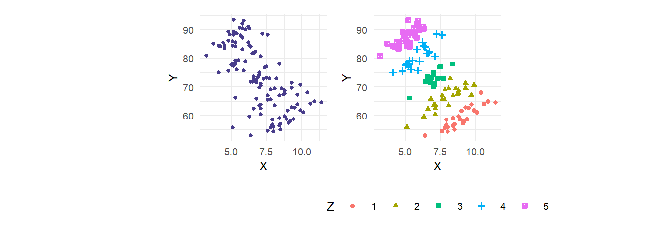
We showed that the multiple linear regression model \[ Y_i = \beta_0 + \beta_1 X_i + \beta_2 Z_i + \epsilon_i\,, \] estimated using OLS, manages to disentangle the effects of \(X\) and \(Z\) on \(Y\). We recreate the regressions from Example 3.3 below, this time including the \(R^2\) measure of goodness-of-fit (see Exercise 3.12).
dat1 <- read_csv("data\\multireg_eg.csv",col_types = c("n","n","n"))
dat1_lm1_sum <- lm(Y~X, data=dat1) %>% summary()
dat1_lm2_sum <- lm(Y~X+Z, data=dat1) %>% summary()
cat("Dependent variable: Y\n\n")
dat1_lm1_sum %>% coefficients %>% round(4);
cat("R-squared:", round(dat1_lm1_sum$r.squared, 3), "\n\n")
dat1_lm2_sum %>% coefficients %>% round(4);
cat("R-squared:", round(dat1_lm2_sum$r.squared, 3))
Dependent variable: Y
Estimate Std. Error t value Pr(>|t|)
(Intercept) 102.8641 3.2199 31.9463 0
X -4.2321 0.4475 -9.4578 0
R-squared: 0.431
Estimate Std. Error t value Pr(>|t|)
(Intercept) 21.1883 2.0817 10.1786 0
X 3.1145 0.2054 15.1602 0
Z 10.1097 0.2380 42.4806 0
R-squared: 0.965How is it that multiple linear regression model (and the OLS estimation of it) manages to disentangle the effects of \(X\) and \(Z\) on \(Y\)? Besides disentangling the effects of multiple factors, notice that the standard error on \(X\) also falls when \(Z\) is added to the regression. Is this always the case? We see that the \(R^2\) goes up. Will this always happen?
Example 4.2 Regressing ln earn on height using data in earnings2019.csv produces the following result:
dat2<-read_csv("data\\earnings2019.csv",show_col_types=FALSE) %>%
  mutate(white=if_else(race=="White", 1,0),
         black=if_else(race=="Black", 1,0),
         other=if_else(race=="Other", 1,0)) %>% select(-race)
dat2_lm1_sum <- summary(lm(log(earn)~height, data=dat2))
dat2_lm1_sum %>% coefficients %>% round(4)
Estimate Std. Error t value Pr(>|t|)
(Intercept) 1.2382 0.1536 8.0617 0
height 0.0284 0.0023 12.4766 0cat("R-squared:", round(dat2_lm1_sum$r.squared, 3))R-squared: 0.031An increase in height of one inch is associated with 2.84 percent increase in average hourly earnings, and the result is statistically significant. Of course, this must surely be another case of omitted factors. In particular, including male changes the estimated relationship between ln earn and height:
dat2_lm2_sum <- summary(lm(log(earn)~height+male, data=dat2))
dat2_lm2_sum %>% coefficients %>% round(4)
Estimate Std. Error t value Pr(>|t|)
(Intercept) 1.8140 0.2003 9.0568 0
height 0.0191 0.0031 6.1896 0
male 0.1109 0.0248 4.4668 0cat("R-squared:", round(dat2_lm2_sum$r.squared, 3))R-squared: 0.034Including male (1 if individual is male, 0 if female) reduces the coefficient on height to 0.0191, suggesting that at least part of the influence of height on ln earn can be explained as a gender gap, the effect of which in the previous regression was attributed to height, since men are taller than women on average. Again, how does OLS estimation of the multiple linear regression manage to disentangle the effects of height and male. The standard error on height goes up with male is added. Why does this happen when in the previous example, the standard error fell when a confounding factor was included?
Is it possible for the coefficient estimate and standard error on one variable to remain essentially unchanged when an important explanatory factor is added? Consider adding age instead of male to the height equation. We get
dat2_lm3_sum <- summary(lm(log(earn)~height+age, data=dat2))
dat2_lm3_sum %>% coefficients %>% round(4)
Estimate Std. Error t value Pr(>|t|)
(Intercept) 0.9072 0.1557 5.8253 0
height 0.0286 0.0023 12.7034 0
age 0.0075 0.0008 9.8971 0cat("R-squared:", round(dat2_lm3_sum$r.squared, 3))R-squared: 0.049Adding age, which is a significant factor, leaves the coefficient on height practically unchanged. When does adding a factor change previous results and when does it not?
Example 4.3 Even if the objective is to estimate the conditional expectation of \(Y\) on a single factor only, the multiple linear regression model can provide additional flexibility in functional form. In the previous chapter, we specified the conditional expectation of \(\ln earn\) given \(educ\) as \[
E(\ln educ \mid educ) = \beta_0 + \beta_1 educ\,.
\] For the data in earnings2019.csv, one might argue that a non-linear specification might be better, especially at lower levels of educ, see Fig. 4.2(a). Using the multiple linear regression framework, we can allow for non-linear specifications of the conditional expectation, such as: \[
E(\ln educ \mid educ) = \beta_0 + \beta_1 educ + \beta_2 educ^2\,.
\] Regressing \(\ln earn\) on \(educ\) and \(educ^2\) does produce a more satisfying fit.
ggplot(dat2, aes(y=log(earn),x=educ)) + geom_point(size=0.5) + scale_x_continuous(breaks=7:17) +
  geom_smooth(formula=y~x+I(x^2), se=FALSE, method="lm") + theme_classic()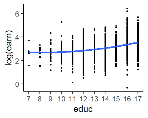
You can also have interaction effects, such as \[ \ln educ = \beta_0 + \beta_1 male + \beta_2 educ + \beta_3 educ . male + \epsilon\,. \] When \(male=0\) the equation becomes \[ \ln educ = \beta_0 + \beta_2 educ + \epsilon \] whereas when \(male=1\), we have \[ \ln educ = \beta_0 + \beta_1 + (\beta_2+\beta_3) educ + \epsilon \] thereby allowing the returns to education parameter (the coefficient on \(educ\)) to depend on the sex of the individual. You might be interested in testing whether \(\beta_3 = 0\) or \(\beta_1 = \beta_3 = 0\). For our dataset, we have:1
dat2_lm4_sum <- summary(lm(log(earn)~educ*male, data=dat2)) ## Note the formula and the output!
dat2_lm4_sum %>% coefficients %>% round(4)
cat("R-squared:", round(dat2_lm4_sum$r.squared, 3))
Estimate Std. Error t value Pr(>|t|)
(Intercept) 0.9645 0.0809 11.9219 0.0000
educ 0.1438 0.0055 26.0461 0.0000
male 0.5353 0.1125 4.7586 0.0000
educ:male -0.0183 0.0078 -2.3510 0.0188
R-squared: 0.217It seems that the returns to education is a little bit lower for men than for women, whereas there is a large gender gap even after controlling for years of education. Males with, say, 10 years of education earn \(53.53-1.83(10) = 35.23\%\) more than women with the same number of years of education. Of course, there are certainly more factors that need to be controlled for.
In this chapter, we focus on ordinary least squares (OLS) estimation of the multiple linear regression with two regressors: \[ Y = \beta_0 + \beta_1 X + \beta_2 Z + \epsilon. \] We focus on the two regressor case in the first instance in order to build intuition regarding issues such as bias-variance tradeoffs, how the inclusion of an additional variable helps to “control” for the confounding effect of that variable, and basic ideas about joint hypotheses testing. We continue to assume that you are working with cross-sectional data. Be reminded that the variables \(Y\), \(X\) and \(Z\) may be transformations of the variables of interest. Furthermore, \(X\) and \(Z\) may be transformations of the same variable, e.g., we may have \(Z = X^2\).
4.2 OLS Estimation of the Multiple Linear Regression Model
Let \(\{Y_{i}, X_{i}, Z_{i}\}_{i=1}^n\) be your sample. For any estimators \(\hat{\beta}_0\), \(\hat{\beta}_1\) and \(\hat{\beta}_2\) (whether or not obtained by OLS), define the fitted values to be \[ \hat{Y}_{i} = \hat{\beta}_{0} + \hat{\beta}_{1} X_{i} + \hat{\beta}_{2} Z_{i} \tag{4.1}\] and the residuals to be \[ \hat{\epsilon}_{i} = Y_{i} - \hat{Y}_{i} = Y_{i} - \hat{\beta}_{0} - \hat{\beta}_{1} X_{i} - \hat{\beta}_{2} Z_{i} \tag{4.2}\] for \(i=1,2,...,n\). The OLS method chooses \((\hat{\beta}_{0}, \hat{\beta}_{1}, \hat{\beta}_{2})\) to be those values that minimize the residual sum of squares \(RSS = \sum_{i=1}^{n} (Y_{i} - \hat{\beta}_{0} - \hat{\beta}_{1} X_{i} - \hat{\beta}_{2} Z_{i})^2\), i.e., \[ {\hat{\beta}_{0}^{ols}, \hat{\beta}_{1}^{ols}, \hat{\beta}_{2}^{ols}} = \text{argmin}_{\hat{\beta}_0, \hat{\beta}_1, \hat{\beta}_2} \sum_{i=1}^n (Y_i - \hat{\beta}_0 - \hat{\beta}_1X_i - \hat{\beta}_2Z_i)^2. \tag{4.3}\] The phrase “\(\text{argmin}_{\hat{\beta}_{0}, \hat{\beta}_{1}, \hat{\beta}_{2}}\)” means “the values of \(\hat{\beta}_{0}, \hat{\beta}_{1}, \hat{\beta}_{2}\) that minimize …”. The OLS estimators can be found by solving the first order conditions for the minimization problem: \[ \begin{aligned} \left.\frac{\partial RSS}{\partial \hat{\beta}_0}\right|_{\hat{\beta}_0^{ols},\hat{\beta}_1^{ols},\hat{\beta}_2^{ols}} &= -2\sum_{i=1}^n(Y_i-\hat{\beta}_0^{ols}-\hat{\beta}_1^{ols}X_i-\hat{\beta}_2^{ols}Z_i)=0\,, \\ \left.\frac{\partial RSS}{\partial \hat{\beta}_1}\right|_{\hat{\beta}_0^{ols},\hat{\beta}_1^{ols},\hat{\beta}_2^{ols}} &= -2\sum_{i=1}^n(Y_i-\hat{\beta}_0^{ols}-\hat{\beta}_1^{ols}X_i-\hat{\beta}_2^{ols}Z_i)X_i=0\,, \\ \left.\frac{\partial RSS}{\partial \hat{\beta}_2}\right|_{\hat{\beta}_0^{ols},\hat{\beta}_1^{ols},\hat{\beta}_2^{ols}} &= -2\sum_{i=1}^n(Y_i-\hat{\beta}_0^{ols}-\hat{\beta}_1^{ols}X_i-\hat{\beta}_2^{ols}Z_i)Z_i=0\,. \end{aligned} \tag{4.4}\] We can also write the first order conditions as2 \[ \sum_{i=1}^n \hat{\epsilon}_i^{ols} = 0\,, \quad \sum_{i=1}^n \hat{\epsilon}_i^{ols}X_i = 0\,, \quad \text{and} \quad \sum_{i=1}^n \hat{\epsilon}_i^{ols}Z_i = 0\,. \tag{4.5}\]
Instead of solving the three-equation three-unknown system (4.4) directly, we are going to take an alternative but entirely equivalent approach. This alternative approach is indirect, but more illustrative. We focus on the estimation of \(\hat{\beta}_{1}^{ols}\). You can get the solution for \(\hat{\beta}_{2}^{ols}\) by switching \(X_{i}\) with \(Z_{i}\) in the steps shown. After obtaining \(\hat{\beta}_{1}^{ols}\) and \(\hat{\beta}_{2}^{ols}\), you can use the first equation in (4.4) to compute \[ \hat{\beta}_{0}^{ols} = \overline{Y} - \hat{\beta}_{1}^{ols}\overline{X} - \hat{\beta}_{2}^{ols}\overline{Z}\,. \] We begin with the following “auxiliary” regressions:
Regress \(X_{i}\) on \(Z_{i}\), and collect the residuals \(r_{i,x \mid z}\) from this regression, i.e., compute \[ r_{i,x \mid z} = X_{i} - \hat{\delta}_{0} - \hat{\delta}_{1} Z_{i} \; , \; i=1,2,...,n \] where \(\hat{\delta}_0\) and \(\hat{\delta}_1\) are the OLS estimators for the intercept and slope coefficients from a regression of \(X_i\) on a constant and \(Z_i\). We can write \[ X_i = \widehat{X}_i + r_{i, x \mid z} \;\text{ where }\; \widehat{X}_i = \widehat{\delta}_0 + \widehat{\delta}_1 Z_i\,,\; i=1,\dots, n\,. \] The fitted values \(\widehat{X}_i\) are perfectly correlated with \(Z_i\), and the residuals \(r_{i, x \mid z}\) are perfectly uncorrelated with \(Z_i\). You can think of this regression as “breaking up” \(X_i\) into two parts, \(\widehat{X}_i\) and \(r_{i, x \mid z}\). The residuals contain the movements in \(X_i\) after filtering out that part of \(X_i\) that is correlated with \(Z_i\).
Regress \(Y_i\) on \(Z_i\), and collect the residuals \(r_{i,y \mid z}\) from this regression, i.e., compute \[ r_{i,y \mid z} = Y_i - \hat{\alpha}_0 - \hat{\alpha}_1Z_i \; , \; i=1,2,...,n \] where \(\hat{\alpha}_0\) and \(\hat{\alpha}_1\) are the OLS estimators for the intercept and slope coefficients from a regression of \(Y_i\) on a constant and \(Z_i\). As in the first regression, the residuals \(r_{i,y \mid z}\) contain the movements in \(Y_i\) after filtering out that part of \(Y_i\) that is correlated with \(Z_i\).
The OLS estimator \(\hat{\beta}_1^{ols}\) obtained from solving the first order conditions (4.4) turns out to be equal to the OLS estimator of the coefficient on \(r_{i,x \mid z}\) in a regression of \(r_{i,y \mid z}\) on \(r_{i,x \mid z}\) (you can exclude the intercept term here; the sample means of both residuals are zero by construction, so the estimator for the intercept term if included will also be zero). In other words, \[ \hat{\beta}_1^{ols} = \frac{\sum_{i=1}^n r_{i,x \mid z}r_{i,y \mid z}}{\sum_{i=1}^n r_{i,x \mid z}^2}. \tag{4.6}\] To see this, note that since \(\{r_{i,x \mid z}\}_{i=1}^n\) are OLS residuals from a regression of \(X_i\) on an intercept term and \(Z_i\), we have \(\sum_{i=1}^n r_{i,x \mid z} = 0\) and \(\sum_{i=1}^n r_{i,x \mid z}Z_i = 0\). This implies \[ \sum_{i=1}^n r_{i,x \mid z}\hat{X}_i = \sum_{i=1}^n r_{i,x \mid z}(\hat{\delta}_0 + \hat{\delta}_1Z_i) = 0 \] and furthermore, \[ \sum_{i=1}^n r_{i,x \mid z}X_i = \sum_{i=1}^n r_{i,x \mid z}(\hat{X}_i + r_{i,x \mid z}) = \sum_{i=1}^n r_{i,x \mid z}^2. \] Now consider the sum \(\sum_{i=1}^n r_{i,x \mid z}r_{i,y \mid z}\). We have \[ \begin{aligned} \sum_{i=1}^n r_{i,x \mid z}r_{i,y \mid z} &= \sum_{i=1}^n r_{i,x \mid z}(Y_i - \hat{\alpha}_0 - \hat{\alpha}_1 Z_i) = \sum_{i=1}^n r_{i,x \mid z}Y_i \\ &= \sum_{i=1}^n r_{i,x \mid z}(\hat{\beta}_0^{ols} + \hat{\beta}_1^{ols}X_i + \hat{\beta}_2^{ols}Z_i + \hat{\epsilon}_i) = \hat{\beta}_1^{ols}\sum_{i=1}^n r_{i,x \mid z}^2 + \sum_{i=1}^n r_{i,x \mid z}\hat{\epsilon}_i. \end{aligned} \tag{4.7}\] Finally, we note that the first order conditions (4.4) imply that \[ \begin{aligned} \sum_{i=1}^n r_{i,x \mid z}\hat{\epsilon}_i &= \sum_{i=1}^n \hat{\epsilon}_i(X_i - \hat{\delta}_0 - \hat{\delta}_1Z_i) \\ &= \sum_{i=1}^n \hat{\epsilon}_iX_i - \hat{\delta}_0\sum_{i=1}^n \hat{\epsilon}_i - \hat{\delta}_1\sum_{i=1}^n \hat{\epsilon}_iZ_i = 0. \end{aligned} \] Therefore \[ \sum_{i=1}^n r_{i,x \mid z}r_{i,y \mid z} = \hat{\beta}_1^{ols}\sum_{i=1}^n r_{i,x \mid z}^2 \] which gives (4.6).
Note that in order for (4.6) to be feasible, we require \(\sum_{i=1}^n r_{i,x \mid z}^2 \neq 0\). This means that \(X_i\) and \(Z_i\) cannot be perfectly correlated. They can be correlated, just not perfectly so. Furthermore, in the auxiliary regression of \(X_i\) on \(Z_i\), we require some variation in \(Z_i\), i.e., it cannot be that all the \(Z_i\), \(i=1,2,...,n\) have the same value \(c\). Similarly, to derive \(\hat{\beta}_2^{ols}\), we require variation in \(X_i\). All this is perfectly intuitive. If there is no variation in \(X_i\) in the sample, we cannot measure how \(Y_i\) changes with \(X_i\). Similarly for \(Z_i\). If \(X_i\) and \(Z_i\) are perfectly correlated, we will not be able to tell whether a change in \(Y_i\) is due to a change in \(X_i\) or in \(Z_i\), since they move in perfect lockstep. We can summarize all of these requirements by saying that we require \[ c_1 + c_2X_i + c_3Z_i = 0\;\text{ for all }\; i=1,2,...,n \;\Longleftrightarrow (c_1,c_2,c_3) = (0,0,0)\,. \] The “\(\Leftarrow\)” implication clearly always holds; that’s not the important part. The important part is the “\(\Rightarrow\)” implication, which does not always hold. In particular, if \(X_i\) or \(Z_i\) take the same value for all \(i=1, \dots, n\), or if \(X_i\) and \(Z_i\) are perfect correlated, then the “\(\Rightarrow\)” implication will not hold. If \(X_i = c\) for all \(i=1, \dots, n\), then set \(c_1 = -c, c_2 = 1, c_3=0\) and we get \(c_1 + c_2X_i + c_3Z_i = -c + c + 0 = 0\) for all \(i=1, \dots, n\). If \(Z_i = c\) for all \(i\), then set \(c_1 = -c, c_2 = 0, c_3=1\). If \(X_i = a + bZ_i\) for all \(i\), (with \(b \neq 0\)) then set \(c_1= -a, c_2 = 1, c_3 = -b\) which gives \(c_1 + c_2X_i + c_3Z_i = -a + a + bZ_i - bZ_i = 0\) for all \(i=1, \dots, n\).
The arguments presented in this section show the essence of how confounding factors are ‘controlled’ in multiple regression analysis. Suppose we want to measure how \(Y_i\) is affected by \(X_i\). If \(Z_i\) is an important determinant of \(Y_i\) that is correlated with \(X_i\), but omitted from the regression, then the measurement of the influence of \(X_i\) on \(Y_i\) will be distorted. In an experiment, we would control for \(Z_i\) by literally holding it fixed when collecting \(X_i\) and \(Y_i\). In applications in economics, this is impossible. What multiple regression analysis does instead is to strip out all variation in \(Y_i\) and \(X_i\) that are correlated with \(Z_i\), and then measure the correlation in the remaining variation between \(Y_i\) and \(X_i\).
4.3 Algebraic Properties of OLS Estimators
We drop the ‘OLS’ superscript in our notation of the OLS estimators, residuals, and fitted values from this point, and write \(\hat{\beta}_0\), \(\hat{\beta}_1\), \(\hat{\beta}_2\), \(\hat{\epsilon}_i\) and \(\hat{Y}_i\) for \(\hat{\beta}_0^{ols}\), \(\hat{\beta}_1^{ols}\), \(\hat{\beta}_2^{ols}\), \(\hat{\epsilon}_i^{ols}\) and \(\hat{Y}_i^{ols}\) respectively. We will reinstate the ‘ols’ superscript whenever we need to emphasize that OLS was used, or when comparing OLS estimators to estimators derived in another way.
Many of the algebraic properties carry over from the simple linear regression model. These properties all come about because the OLS estimators satisfy the first order conditions \[ \sum_{i=1}^n \hat{\epsilon}_i=0, \quad \sum_{i=1}^n X_i \hat{\epsilon}_i =0 \quad \text{and} \quad \sum_{i=1}^n Z_i \hat{\epsilon}_i =0. \]
This implies that the fitted values \(\hat{Y}_i\) and the residuals are also uncorrelated.
The point \((\overline{X},\overline{Y},\overline{Z})\) always lies on the estimate regression function.
We continue to have \(\overline{Y} = \overline{\hat{Y}}\).
The \(TSS = FSS + RSS\) equality continues to hold in the multiple regression case \[ \sum_{i=1}^n (Y_i - \overline{Y})^2 = \sum_{i=1}^n (\hat{Y}_i - \overline{\hat{Y}})^2 + \sum_{i=1}^n \hat{\epsilon}_i^2. \tag{4.8}\]
As in the simple linear regression case, we can use (4.8) to define the goodness-of-fit measure: \[ R^2 = 1 - \frac{RSS}{TSS}. \tag{4.9}\] It should be noted that the \(R^2\) will never decrease as we add more variables into the regression. This is because OLS minimizes \(RSS\), and therefore maximizes \(R^2\). For example, the \(R^2\) from the regression \(Y = \beta_0 + \beta_1X + \beta_2Z + u\) will never be less than the \(R^2\) from the regression \(Y = \alpha_0 + \alpha_1X + \epsilon\), and will generally be greater, unless it so happens that \(\hat{\beta}_0 = \hat{\alpha}_0\), \(\hat{\beta}_1 = \hat{\alpha}_1\) and \(\hat{\beta}_2 = 0\). If \(\hat{\beta}_1\), \(\hat{\beta}_2\) or \(\hat{\beta}_3\) take on any other value, it will be because the RSS can be further minimized, and the \(R^2\) made larger. For this reason, the “Adjusted \(R^2\)” \[ \text{Adj.-}R^2 = 1 - \frac{\frac{1}{n-K}RSS}{\frac{1}{n-1}TSS} \] is sometimes used, where \(K\) is the number of coefficients estimated (including the intercept term; for the 2-regressor case that we are focusing on, \(K=3\)). The idea is to use unbiased estimates of the variances of \(\epsilon_i\) and \(Y_i\) in computing the goodness-of-fit. Since both \(RSS\) and \(n-K\) decrease when additional variables (and parameters) are added into the model, the adjusted \(R^2\) will increase only if \(RSS\) falls enough to lower the value of \(RSS/(n-k)\). The adjusted \(R^2\) may be used as an alternate measure of goodness-of-fit, but it should not be used as a model selection tool, for reasons we shall come to in a later chapter.
In the derivation (4.7) of the OLS estimator \(\hat{\beta}_1\), we noted that \[ \begin{aligned} \sum_{i=1}^n r_{i,x \mid z}r_{i,y \mid z} &= \sum_{i=1}^n r_{i,x \mid z}(Y_i - \hat{\alpha}_0 - \hat{\alpha}_1 Z_i) \\ &= \sum_{i=1}^n r_{i,x \mid z}Y_i. \end{aligned} \] This implies that the estimator can also be written as \[ \hat{\beta}_1 = \frac{\sum_{i=1}^n r_{i,x \mid z}r_{i,y \mid z}}{\sum_{i=1}^n r_{i,x \mid z}^2} = \frac{\sum_{i=1}^n r_{i,x \mid z}Y_i}{\sum_{i=1}^n r_{i,x \mid z}^2} \tag{4.10}\] which is the formula for the simple linear regression of \(Y_i\) on \(r_{i,x \mid z}\). In other words, you can also get the OLS estimator \(\hat{\beta}_1\) by regressing \(Y_i\) on \(r_{i,x \mid z}\) without first stripping out the covariance between \(Y_i\) and \(Z_i\). Equation (4.10), however, does not fully reflect what happens in a regression of \(Y_i\) on two regressors.
The expression (4.10) shows that \(\hat{\beta}_1\) is a linear estimator, i.e., \[ \hat{\beta}_1 = \sum_{i=1}^n w_i Y_i \] where the weights here are \(w_i = r_{i,x \mid z}/\sum_{i=1}^n r_{i,x \mid z}^2\). Note that the weights \(w_i\) are made up solely of observations \(\{X_i\}_{i=1}^n\) and \(\{Z_i\}_{i=1}^n\), since they are the residuals from a regression of \(X_i\) on \(Z_i\). Furthermore, the weights have the following properties: \[ \begin{aligned} & \sum_{i=1}^n w_i = 0\,, \\ & \sum_{i=1}^n w_iZ_i = \frac{\sum_{i=1}^nr_{i,x \mid z}Z_i}{\sum_{i=1}^nr_{i,x \mid z}^2} = 0 \,, \\ & \sum_{i=1}^n w_iX_i = \frac{\sum_{i=1}^nr_{i,x \mid z}X_i}{\sum_{i=1}^nr_{i,x \mid z}^2} = 1 \,, \\ & \sum_{i=1}^n w_i^2 = \frac{\sum_{i=1}^nr_{i,x \mid z}^2}{(\sum_{i=1}^nr_{i,x \mid z}^2)^2} = \frac{1}{\sum_{i=1}^nr_{i,x \mid z}^2} \,. \end{aligned} \]
If the sample correlation between \(X_i\) and \(Z_i\) is zero, then the coefficient estimate \(\hat{\delta}_1\) in the auxiliary regression where we regressed \(X\) on \(Z\) would be zero, and \(\hat{\delta}_0\) would be equal to the sample mean of \(\overline{X}\). In other words, we would have \(r_{i,x \mid z} = X_i - \overline{X}\), so \[ \hat{\beta}_1 = \frac{\sum_{i=1}^n r_{i,x \mid z}Y_i}{\sum_{i=1}^n r_{i,x \mid z}^2} = \frac{\sum_{i=1}^n (X_i - \overline{X})Y_i}{\sum_{i=1}^n (X_i - \overline{X})^2} \] This is, of course, just the OLS estimator for the coefficient on \(X_i\) in the simple linear regression of \(Y\) on \(X\). In other words, if the sample correlation between \(X_i\) and \(Z_i\) is zero, then including \(Z_i\) in the regression would not change the value of the simple linear regression estimator for the coefficient on \(X_i\). We will see shortly that including the additional variable may nonetheless still reduce the estimator variance.
4.4 Statistical Properties of OLS Estimators
The assumption that \(E(\epsilon \mid X, Z) = 0\) in population, and that we have a representative i.i.d. sample from the population, leads to the following (which we will also call “assumptions”):
(A1) \(E(\epsilon_i \mid \text{x}, \text{z}) = 0\) for all \(i=1,...,n\),
(A2) \(E(\epsilon_i\epsilon_j \mid \text{x}, \text{z}) = 0\) for all \(i\neq j, \; i,j=1,...,n\) where \(\text{x}\) denotes \(X_1,X_2,...,X_n\), and \(\text{z}\) to denotes \(Z_1,Z_2,...,Z_n\).
We will also assume homoskedastic errors
(A3) \(E(\epsilon_i^2 \mid \text{x}, \text{z}) = \sigma^2\) for all \(i=1,...,n\).
Assumption (A1) in particular, leads to unbiased OLS estimators. To see this, first write \[ \hat{\beta}_1 = \sum_{i=1}^n w_i Y_i = \sum_{i=1}^n w_i(\beta_0 + \beta_1X_i + \beta_2 Z_i + \epsilon_i) = \beta_1 + \sum_{i=1}^n w_i \epsilon_i\,. \] Taking conditional expectations. noting that the weights \(w_i\) comprise only \(\text{x}\) and \(\text{z}\), gives \[ E(\hat{\beta}_1 \mid \text{x}, \text{z}) = \beta_1 + \sum_{i=1}^n w_i E(\epsilon_i \mid \text{x}, \text{z}) = \beta_1\,. \] It follows that the unconditional mean is \(E(\hat{\beta}_1) = \beta_1\).
The conditional variance of \(\hat{\beta}_1\) under our assumptions is \[ \begin{aligned} \mathit{Var}(\hat{\beta_1} \mid \text{x}, \text{z}) &= \mathit{Var}\left(\left.\beta_1+\sum_{i=1}^n w_i\epsilon_i \;\right|\; \text{x}, \text{z}\right) \\ &= \sum_{i=1}^n w_i^2\mathit{Var}(\epsilon_i \mid \text{x}, \text{z}) \\ &= \frac{\sigma^2}{\sum_{i=1}^nr_{i,x \mid z}^2}\,. \end{aligned} \tag{4.11}\] Since the \(R^2\) from the regression of \(X_i\) on \(Z_i\) is \[ R_{x \mid z}^2 = 1 - \frac{\sum_{i=1}^nr_{i,x \mid z}^2}{\sum_{i=1}^n(X_i - \overline{X})^2}\,, \] we can also write \(\mathit{Var}(\hat{\beta_1} \mid \text{x}, \text{z})\) as \[ \mathit{Var}(\hat{\beta_1} \mid \text{x}, \text{z}) = \frac{\sigma^2}{(1-R_{x \mid z}^2)\sum_{i=1}^n(X_i-\overline{X})^2}\,. \tag{4.12}\]
Expression (4.12) clearly shows the trade-offs involved in adding a second regressor. Suppose the true data generating process is \[ Y = \beta_0 + \beta_1 X + \beta_2 Z + \epsilon \,,\; E(\epsilon \mid X, Z) = 0 \] but you ran the regression \[ Y = \beta_0 + \beta_1 X + u. \] If \(X\) and \(Z\) are correlated, then \(X\) and \(u\) are correlated, and you will get biased estimates of \(\beta_1\). By estimating the multiple linear regression, you are able to get an unbiased estimate of \(\beta_1\) by controlling for \(Z\). However, the variance of the OLS estimator for \(\beta_1\) changes from \[ \mathit{Var}(\hat{\beta_1} \mid \text{x}) = \frac{\sigma_u^2}{\sum_{i=1}^n(X_i-\overline{X})^2} \] in the simple linear regression to the expression in (4.12) for the multiple linear regression. Since \(\sigma^2\) is the variance of \(\epsilon\), and \(\sigma_u^2\) is the variance of a combination of the uncorrelated variables \(Z\) and \(\epsilon\), we have \(\sigma^2 < \sigma_u^2\). This has the effect of reducing the estimator variance (which is good!). However, since \(0 < 1-R_{x \mid z}^2 < 1\), the denominator in the variance expression is smaller in the multiple linear regression case than in the simple linear regression case. This is because in the multiple regression, we have stripped out all variation in \(X\) that is correlated with \(Z\), resulting in reduced effective variation in \(X\), which in turn increases the estimator variance. In general (and especially in causal applications), one would usually consider the trade-off to be in favor of the multiple regression. However, if \(X\) and \(Z\) are highly correlated (\(R_{x \mid z}^2\) close to 1), then the reduction in effective variation in \(X\) may be so severe that the estimator variance becomes very large. This tends to reduce the size of the t-statistic, leading to rejection of statistical significance even in cases where the size of the estimate itself may suggest strong economic significance.
To compute a numerical estimate for the conditional variance of \(\hat{\beta}_1\), we have to estimate \(\sigma^2\). An unbiased estimator for \(\sigma^2\) in the two-regressor case is \[ \widehat{\sigma^2} = \frac{1}{n-3}\sum_{i=1}^n \hat{\epsilon}_i^2. \tag{4.13}\] The \(RSS\) is divided by \(n-3\) because three “degrees-of-freedom” were used in computing \(\hat{\beta}_0\), \(\hat{\beta}_1\) and \(\hat{\beta}_2\) and these were used in the computation of \(\hat{\epsilon}_i\). We shall again leave the proof of unbiasedness of \(\widehat{\sigma^2}\) for when we deal with the general case. We estimate the conditional variance of \(\hat{\beta}_1\) using \[ \widehat{\mathit{Var}}(\hat{\beta}_1 \mid \mathrm{x},\mathrm{z}) = \frac{\widehat{\sigma^2}}{(1-R_{x \mid z}^2)\sum_{i=1}^n(X_i - \overline{X})^2} \tag{4.14}\] The standard error of \(\hat{\beta}_1\) is the square root of (4.14).
Example 4.4 We illustrate the main points of this chapter using our multireg_eg.csv dataset, reproduced yet again below as Fig. 4.3.
df <- read_csv("data\\multireg_eg.csv",col_types = c("n","n","n"))
p1 <- ggplot(data=df) + geom_point(aes(x=X, y=Y), color="darkslateblue") + theme_minimal() + theme1
p2 <- ggplot(data=df) + geom_point(aes(x=X, y=Y, shape=as.factor(Z), color=as.factor(Z))) +
      theme_minimal() + theme2 + labs(shape='Z', color='Z')
p1|p2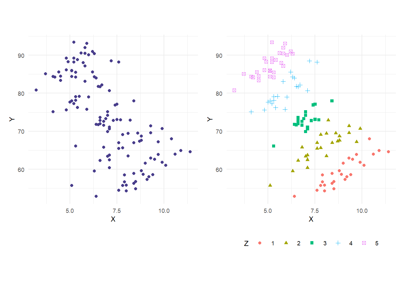
We run two regressions below. The first is a simple linear regression of \(Y\) on \(X\). The second is a multiple linear regression of \(Y\) on \(X\) and \(Z\).
mdl1 <- lm(Y~X, data=df)
coef(summary(mdl1))
cat("R-squared:", summary(mdl1)$r.squared,"\n\n")
Estimate Std. Error t value Pr(>|t|)
(Intercept) 102.86406 3.2199095 31.94626 6.373574e-60
X -4.23213 0.4474755 -9.45779 3.857133e-16
R-squared: 0.4311877 mdl2 <- lm(Y~X+Z, data=df)
coef(summary(mdl2))
cat("R-squared:", summary(mdl2)$r.squared,"\n\n") Estimate Std. Error t value Pr(>|t|)
(Intercept) 21.188337 2.0816539 10.17861 8.212834e-18
X 3.114465 0.2054364 15.16024 2.219609e-29
Z 10.109717 0.2379845 42.48057 5.955647e-73
R-squared: 0.9653668 The simple linear regression shows the negative relationship between \(Y\) and \(X\) when viewed over all outcomes of \(Z\). The multiple regression disentangles the effect of \(X\) and \(Z\) on \(Y\). In this case, inclusion of \(Z\) has also substantially reduced the standard error on the estimate of the coefficient on \(X\). As expected, the \(R^2\) has gone up with the inclusion of \(Z\), in this case by a very large amount.
We replicate below the multi-step approach to obtaining the coefficient estimate on \(X\):
mdl1a <- lm(Y~Z, data=df)
r_yz <- residuals(mdl1a)
mdl1b <- lm(X~Z, data=df)
r_xz <- residuals(mdl1b)
df$r_yz <- r_yz
df$r_xz <- r_xz
coef(summary(lm(r_yz~r_xz-1, data=df)))  # "-1" in the formula means exclude the intercept
Estimate Std. Error t value Pr(>|t|)
r_xz 3.114465 0.2037027 15.28926 7.425184e-30The numerical estimate of the coefficient on r_xz is identical to that on X in the previous regression. The standard errors are similar, but not the same. We emphasize that the auxiliary regression approach is for illustrative purposes only. The standard errors, t-statistic, etc. should all be taken from the previous (multiple) regression. The plots in Fig. 4.4 illustrate the effect of ‘controlling’ for Z.
plot_theme <- theme_minimal() + theme(legend.position = "none", plot.title=element_text(size=10))
p1 <- ggplot(data=df) + geom_point(aes(x=X,y=Y, shape=as.factor(Z), color=as.factor(Z))) +
  xlim(c(2.5,12.5)) + ylim(c(50,100)) + ggtitle('(a)') + plot_theme
p2 <- ggplot(data=df) + geom_point(aes(x=r_xz,y=Y, shape=as.factor(Z), color=as.factor(Z))) +
  xlim(c(-5,5)) + ylim(c(50,100)) + ggtitle('(b)') + plot_theme
p3 <- ggplot(data=df) + geom_point(aes(x=r_xz,y=r_yz, shape=as.factor(Z), color=as.factor(Z))) +
  xlim(c(-5,5)) + ylim(c(-25,25)) + ggtitle('(c)') + plot_theme
p1|p2|p3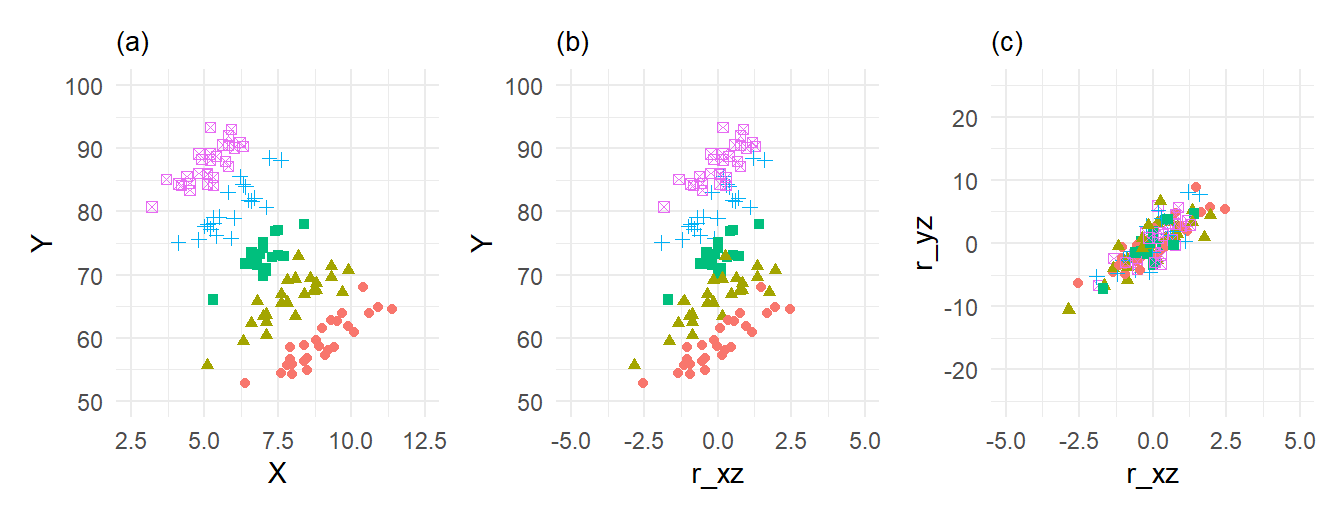
The range of the y-axis in the three plots are the same (50 to 100 in the first two, -25 to 25 in the third). Likewise the range of the x-axis is the same across all three plots (2.5 to 12.5 in the first, -5 to 5 in the second and third). When we regress \(X\) on \(Z\) and take the residuals, we remove the effect of \(Z\) on \(X\) and also center the residuals around zero (OLS residuals always have sample mean zero). You can see from the second diagram that the variation in \(X\) is reduced, which tends to increase the \(X\) coefficient estimator variance. You can also see that the positive relationship between \(Y\) and \(X\) controlling for \(Z\) already shows up, albeit with a lot of noise. By also removing the effect of \(Z\) on \(Y\) (which we do when we include \(Z\) in the regression), we reduce the variation of \(Y\), compare (b) and (c). This reduces the estimator variance. In this example, the reduction in the variation on \(Y\) is very large relative the reduced variation in \(X\), so the overall effect is that the variance on \(\widehat{\beta}_1\) falls. The slope coefficient in the simple regression of the residuals \(r_{i, y \mid z}\) on \(r_{i, x \mid z}\) in the last panel gives the effect of \(X\) on \(Y\), controlling for \(Z\).
4.5 Hypothesis Testing
To test if \(\beta_k\) is equal to some value \(r_k\) in population, we can again use the t-statistic as in the simple linear regression case: \[ t = \frac{\hat{\beta}_k - r_k}{\sqrt{\widehat{\mathit{Var}}(\hat{\beta}_k)}}\,. \tag{4.15}\] If the noise terms are conditionally normally distributed, then the \(t\)-statistic has the t-distribution, with degrees-of-freedom \(n-K\) where \(K=3\) in the two-regressor case with intercept. If we do not assume normality of the noise terms, then (as long as the necessary CLTs apply) we use instead the approximate test, using the \(t\)-statistic as defined above, but using the rejection region derived from the standard normal distribution. You can also test whether a linear combination of the parameters are equal to some value. For example, in the regression \[ Y = \beta_0 + \beta_1 X + \beta_2 Z + \epsilon \] you may wish to test, say, \(H_0: a_1\beta_1 + a_2\beta_2 = r_1 \text{ vs } H_A: a_1\beta_1 + a_2\beta_2 \neq r_1\).
Example 4.5 Suppose the production technology of a firm can be characterized by the Cobb-Douglas production function: \[ Q(L,K) = AL^\alpha K^\beta \] where \(Q(L,K)\) is the quantity produced using \(L\) units of labor and \(K\) units of capital. The constants \(A\), \(\alpha\) and \(\beta\) are the parameters of the model. If we multiply the amount of labor and capital by \(c\), we get \[ Q(cL,cK) = A(cL)^\alpha (cK)^\beta = c^{\alpha+\beta}AL^\alpha K^\beta. \] The sum \(\alpha + \beta\) therefore represents the “returns to scale”. If \(\alpha + \beta = 1\), then there is constant returns to scale, e.g., doubling the amount of labor and capital (\(c=2\)) results in the doubling of total production. If \(\alpha + \beta > 1\) then there is increasing returns to scale, and if \(\alpha + \beta < 1\), we have decreasing returns to scale. A logarithmic transformation of the production function gives \[ \ln Q = \ln A + \alpha \ln L + \beta \ln K. \] If we have observations \(\{Q_i, L_i, K_i\}_{i=1}^n\) of the quantities produced and amount of labor and capital employed by a set of similar firms in an industry, we could estimate the production function for that industry using the regression \[ \ln Q_i = \ln A + \alpha \ln L_i + \beta \ln K_i + \epsilon_i\,. \] A test for constant returns to scale would be the test \(H_0: \alpha + \beta = 1 \text{ vs } H_A: \alpha + \beta \neq 1\).
The \(t\)-statistic for testing a hypothesis such as \[ H_0 : a_1\beta_1 + a_2\beta_2 = r_1 \;\text{ vs }\; H_0 : a_1\beta_1 + a_2\beta_2 \neq r_1 \] is \[ t = \frac{a_1\hat{\beta}_1 + a_2\hat{\beta}_2 - r_1}{\sqrt{\widehat{\mathit{Var}}(a_1\hat{\beta}_1+a_2\hat{\beta}_2)}}. \tag{4.16}\] To compute this \(t\)-statistic you will need an estimate of the covariance of \(\hat{\beta}_1\) and \(\hat{\beta}_2\), the derivation of which we leave for a later chapter. There are packages, of course, that will help you carry out this hypothesis test. For now, we consider an alternative way of forcing your linear regression to provide you with the relevant \(t\)-statistic, which is to re-parameterize your equation. For example, to test the hypothesis \(H_0: \beta_1 + \beta_2 = 1\), we can reparameterize the regression equation as follows: \[ \begin{gathered} Y = \beta_0 + \beta_1 X + \beta_2 Z + \epsilon \\[1ex] Y = \beta_0 + \beta_1 X + \beta_2 X - X + X - \beta_2 X + \beta_2 Z + \epsilon \\[1ex] Y-X = \beta_0 + (\beta_1 + \beta_2 - 1) X + \beta_2 (Z-X) + \epsilon \end{gathered} \] By regressing \(Y-X\) on \(X\) and \(Z-X\) (and an intercept), you can test \(H_0: \beta_1 + \beta_2 = 1\) by testing if the coefficient on \(X\) is equal to zero.
Example 4.6 Using data in the earnings2019.xlsx, we estimate the regression \[
\ln earn = \beta_0 + \beta_1 educ + \beta_2 black + \beta_3 female + \beta_4 black.female+ \epsilon\,.
\] To test the hypothesis \(H_0: \beta_2 = \beta_3\) (equivalent to \(H_0: \beta_2 - \beta_3 = 0\)), we re-parameterize the regression equation as \[
\ln earn = \beta_0 + \beta_1 educ + (\beta_2-\beta_3) black + \beta_3 (female+black) + \beta_4 black.female+ \epsilon\,.
\]
dat2$female <- 1 - dat2$male
mdl_earnings1 <- lm(log(earn) ~ educ + black*female, data=dat2)
mdl_earnings1 %>% summary %>% coefficients %>% round(4)
Estimate Std. Error t value Pr(>|t|)
(Intercept) 1.5369 0.0571 26.9219 0.0000
educ 0.1279 0.0039 32.9577 0.0000
black -0.2600 0.0270 -9.6468 0.0000
female -0.2807 0.0196 -14.3238 0.0000
black:female 0.0873 0.0355 2.4601 0.0139mdl_earnings2 <- lm(log(earn) ~ educ + black + I(female+black) + female:black, data=dat2)
mdl_earnings2 %>% summary %>% coefficients %>% round(4) Estimate Std. Error t value Pr(>|t|)
(Intercept) 1.5369 0.0571 26.9219 0.0000
educ 0.1279 0.0039 32.9577 0.0000
black 0.0206 0.0271 0.7607 0.4469
I(female + black) -0.2807 0.0196 -14.3238 0.0000
black:female 0.0873 0.0355 2.4601 0.0139The hypothesis is not rejected.
In some cases, we may wish to test multiple hypotheses, e.g., in the two-variable regression, we may wish to test \[ H_0: \beta_1 = 0 \; \text{ and } \; \beta_2 = 0 \; \text{ vs } \; H_A: \beta_1 \neq 0 \;\text{or}\; \beta_2 \neq 0. \] One possibility would be to do individual \(t\)-tests for each of the two hypotheses, but we should be aware that two individual 5% tests is not equivalent to a joint 5% test. The following example illustrates this problem.
Example 4.7 We generate 100 observations of three uncorrelated variables \(X\), \(Y\) and \(Z\). We regress \(Y\) on \(X\) and \(Z\), and collect the t-statistics on \(X\) and \(Z\). We repeat the experiment 1000 times (with different draws each time, of course, but the same parameters).
set.seed(3)
nreps <- 1000
tx <- tz <- rep(NA,nreps)
n <- 100
for (i in 1:nreps){
  X <- rnorm(n, mean=0, sd=2)
  Z <- rnorm(n, mean=0, sd=2)
  Y <- rnorm(n, mean=0, sd=2)
  df_test <- data.frame(X,Y,Z)
  mdlsim <- lm(Y~X+Z, data=df_test)
  tx[i] <- coef(summary(mdlsim))[2,'t value']
  tz[i] <- coef(summary(mdlsim))[3,'t value']
}
rjt_x <- sum(tx<qt(0.025,n-3) | tx>qt(0.975,n-3))/nreps
cat("Freq. of rejection of Beta_X = 0:", rjt_x, "\n")
Freq. of rejection of Beta_X = 0: 0.058 rjt_z <- sum(tz<qt(0.025,n-3) | tz>qt(0.975,n-3))/nreps
cat("Freq. of rejection of Beta_Z = 0:", rjt_z, "\n")Freq. of rejection of Beta_Z = 0: 0.054 rjt_x_or_z <- sum(tz<qt(0.025,197) | tz>qt(0.975,197) |
tx<qt(0.025,197) | tx>qt(0.975,197))/nreps
cat("Freq. of rejection of Beta_X = 0 and Beta_Z = 0 using two t-tests:", rjt_x_or_z, "\n")Freq. of rejection of Beta_X = 0 and Beta_Z = 0 using two t-tests: 0.112 When using a 5% t-test, we reject the (true) hypothesis that \(\beta_x = 0\) in about 6% of the experiments, close to 5%. These rejections are regardless of whether the t-test for \(\beta_z=0\) rejects or does not reject. Likewise, the 5% t-test for \(\beta_z = 0\) rejects the hypothesis 5.5% of the time, roughly five percent. However, if we say we reject \(\beta_x = 0\) and \(\beta_z = 0\) if either t-tests rejects the corresponding hypothesis, then the frequency of rejection is much larger, roughly double.
We plot the t-stats below, indicating the critical values for the individual tests. The proportion of points above the upper horizontal line or below the lower one is about 0.05. Similarly, the proportion of points to the left of the left vertical line or to the right of the right one is roughly 0.05. The number of point that meet either of the two sets of criteria is much larger, roughly the sum of the two proportions.
df_t <- data.frame(tx,tz)
ggplot(data=df_t) + geom_point(aes(x=tx,y=tz)) +
  geom_hline(yintercept = qt(0.025,n-3), lty='dashed', col='blue') +
  geom_hline(yintercept = qt(0.975,n-3), lty='dashed', col='blue') +
  geom_vline(xintercept = qt(0.025,n-3), lty='dashed', col='blue') +
  geom_vline(xintercept = qt(0.975,n-3), lty='dashed', col='blue') +
  theme_minimal()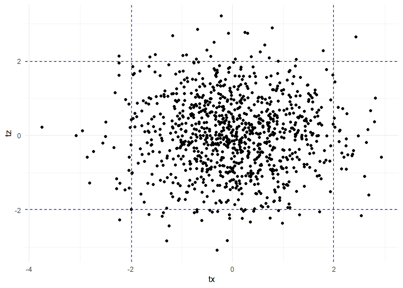
To jointly test multiple hypotheses, we can use the \(F\)-test. Suppose in the regression \[ Y = \beta_0 + \beta_1X + \beta_2 Z + \epsilon \] we wish to jointly test the hypotheses \[ H_0: \beta_1 = 1 \; \text{ and } \; \beta_2 = 0 \; \text{ vs } \; H_A: \beta_1 \neq 1 \;\text{or}\; \beta_2 \neq 0 \;\text{ (or both)}\,. \] Suppose we run the regression twice, once unrestricted, and another time with the restrictions in \(H_0\) imposed. The regression with the restrictions imposed is \[ Y = \beta_0 + X + \epsilon \] so the restricted OLS estimator for \(\beta_0\) is the sample mean of \(Y_i - X_i\), i.e., \[ \hat{\beta}_{0}^{rols} = (1/n)\sum_{i=1}^n(Y_i - X_i). \] Calculate the \(RSS\) from both equations. The “unrestricted \(RSS\)” and “restricted \(RSS\)” are \[ RSS_{ur} = \sum_{i=1}^n \hat{\epsilon}_i^2 \;\;\text{ and }\;\;RSS_{r} = \sum_{i=1}^n \hat{\epsilon}_{i,\,rols}^2 \] respectively, where \(\hat{\epsilon}_i = Y_i - \hat{\beta}_0 - \hat{\beta}_1X_i - \hat{\beta}_2 Z_i\) and \(\hat{\epsilon}_{i,rols} = Y_i - \hat{\beta}_{0}^{rols} - X_i\). Since OLS minimizes \(RSS\), imposing restrictions never decrease \(RSS\), i.e., \[ RSS_r \geq RSS_{ur} \,. \] It can be shown that if the hypotheses in \(H_0\) are true (and the noise terms are normally distributed), then \[ F = \frac{(RSS_r - RSS_{ur})/J}{RSS_{ur}/(n-K)} \sim F{(J,n-K)} \tag{4.17}\] where \(J\) is the number of restrictions being tested (in our example, \(J=2\)) and \(K\) is the number of coefficients to be estimated (including intercept; in our example, \(K=3\)).
The \(F\)-statistic is always non-negative. The idea is that if the hypotheses in \(H_0\) are true in population, then imposing the restrictions on the regression would not increase the \(RSS\) by much (since the unrestricted parameter estimates should be close to their population values), and the \(F\)-statistic will be close to zero. On the other hand, if one or more of the hypotheses in \(H_0\) are false in population, then imposing them onto the regression will cause the \(RSS\) to increase substantially, and the \(F\)-statistic will be large. We take a very large \(F\)-statistic, meaning \[ F > \text{F}_{1-\alpha}(J,n-K)\,, \] as statistical evidence that one or more of the hypothesis is false, where \(\text{F}_{1-\alpha}(J,n-K)\) is the \((1-\alpha)\)-percentile of the \(\text{F}{(J,n-K)}\) distribution and where \(\alpha\) is typically 0.10, 0.05 or 0.01,
Since \(R^2 = 1 - RSS/TSS\), we can write the \(F\)-statistic in terms of \(R^2\) instead of \(RSS\). You are asked in an exercise to show that the \(F\)-statistic can be written as \[ F = \frac{(R_{ur}^2 -R_r^2)/J}{(1-R_{ur}^2)/(n-K)}. \] Imposing restrictions cannot increase \(R^2\), and in general will decrease it. The \(F\)-test essentially tests if the \(R^2\) drops significantly when the restrictions are imposed. If the hypotheses being tested are true, then the drop should be slight. If one or more are false, the drop should be substantial, resulting in a large \(F\)-statistic.
If you cannot assume that the noise terms are conditionally normally distributed, then you will have to use an asymptotic approximation. It can be shown that \[ JF \overset{d}\rightarrow \chi^2{(J)} \] as \(n \rightarrow \infty\), where \(J\) is the number of hypotheses being jointly tested, and \(F\) is the \(F\)-statistic (4.17). We refer to this as the “Chi-square Test”.
Example 4.8 We continue with Example 4.4, which considered the regression \[ \ln earn = \beta_0 + \beta_1 educ + \beta_2 black + \beta_3 female + \beta_4 black.female+ \epsilon\,. \] This time we test the hypothesis \(H_0: \beta_2 = \beta_3\) and \(\beta_4 = 0\), vs the alternative that at least one of these two restrictions do not hold in population. The restricted regression is \[ \begin{aligned} \ln earn &= \beta_0 + \beta_1 educ + \beta_2 black + \beta_2 female + 0 black.female+ \epsilon \\ &= \beta_0 + \beta_1 educ + \beta_2 (black + female) + \epsilon \end{aligned} \] We carry out the \(F\)-test of our hypotheses below:
mdl_unres <- lm(log(earn) ~ educ + black*female, data=dat2)
mdl_res <- lm(log(earn) ~ educ + I(black + female), data=dat2)
RSS_unres <- sum(residuals(mdl_unres)^2)
RSS_res   <- sum(residuals(mdl_res)^2)
J = 2
n_minus_K <- mdl_unres$df.residual
Fstat = ((RSS_res - RSS_unres) / J) / (RSS_unres / n_minus_K)
pval = 1-pf(Fstat, J, n_minus_K)
cat("F-stat:", Fstat, "   pvalue:", pval)
F-stat: 4.546114 pvalue: 0.01065276The joint hypothesis is rejected (at 0.05 significance level, but not 0.01 significance level).
We can use the function linearHypothesis() from the car package to carry out F tests.
mdl_unres <- lm(log(earn) ~ educ + black*female, data=dat2)
linearHypothesis(mdl_unres, c("black=female", "black:female=0"))
Linear hypothesis test:
black - female = 0
black:female = 0

Model 1: restricted model
Model 2: log(earn) ~ educ + black * female

  Res.Df    RSS Df Sum of Sq      F  Pr(>F)
1   4943 1606.5
2   4941 1603.5  2    2.9507 4.5461 0.01065 *
---
Signif. codes:  0 '***' 0.001 '**' 0.01 '*' 0.05 '.' 0.1 ' ' 1
To get the chi-square version of the test:
linearHypothesis(mdl_unres, c("black=female", "black:female=0"), test="Chisq")
Linear hypothesis test:
black - female = 0
black:female = 0

Model 1: restricted model
Model 2: log(earn) ~ educ + black * female

  Res.Df    RSS Df Sum of Sq  Chisq Pr(>Chisq)
1   4943 1606.5
2   4941 1603.5  2    2.9507 9.0922    0.01061 *
---
Signif. codes:  0 '***' 0.001 '**' 0.01 '*' 0.05 '.' 0.1 ' ' 1
As you can see, the chi-square statistic is just \(J\) times the \(F\) statistic.
You can use the \(F\)-test to test a single hypothesis, e.g., to test \(\beta_2 = \beta_3\):
linearHypothesis(mdl_unres, c("black=female"))
Linear hypothesis test:
black - female = 0

Model 1: restricted model
Model 2: log(earn) ~ educ + black * female

  Res.Df    RSS Df Sum of Sq      F Pr(>F)
1   4942 1603.7
2   4941 1603.5  1   0.18778 0.5786 0.4469
Notice that the \(F\)-statistic for testing this single hypothesis is just twice that of the \(t\)-statistic for the same hypothesis in Example 4.4 (we will prove this to be the case in general in a later chapter). The p-value is the same.
Finally we note that the summary() output of an lm object contains a \(F\)-statistic. This is the \(F\)-statistic to test the joint hypotheses that all of the coefficients in the regression (not including the intercept) are zero, versus the alternative that at least one of those coefficients are not zero. The output also contains the adjusted \(R^2\) for the estimated regression.
mdl_unres %>% summary()
Call:
lm(formula = log(earn) ~ educ + black * female, data = dat2)

Residuals:
    Min      1Q  Median      3Q     Max
-3.5992 -0.3448  0.0022  0.3515  2.8614

Coefficients:
              Estimate Std. Error t value Pr(>|t|)
(Intercept)   1.536856   0.057086  26.922   <2e-16 ***
educ          0.127858   0.003879  32.958   <2e-16 ***
black        -0.260050   0.026957  -9.647   <2e-16 ***
female       -0.280661   0.019594 -14.324   <2e-16 ***
black:female  0.087299   0.035486   2.460   0.0139 *
---
Signif. codes:  0 '***' 0.001 '**' 0.01 '*' 0.05 '.' 0.1 ' ' 1

Residual standard error: 0.5697 on 4941 degrees of freedom
Multiple R-squared:  0.2389,    Adjusted R-squared:  0.2383
F-statistic: 387.7 on 4 and 4941 DF,  p-value: < 2.2e-16
4.6 Exercises
Exercise 4.1 What is the main conceptual difference between the regressions \[ \begin{aligned} \text{(A)}\qquad& \ln earn = \beta_0 + \beta_1 educ + \beta_2 black + \beta_3 female + \beta_4 black.female+ \epsilon\\[1ex] \text{(B)}\qquad& \ln earn = \beta_0 + \beta_1 educ + \beta_2 black + \beta_3 female + \epsilon\,. \end{aligned} \] In particular, what does the inclusion of the interaction term \(black.female\) in model A allow us to capture that model B does not.
Exercise 4.2 Suppose your estimated sample regression function is \[ \widehat{log(earn)} = 1.35 + 0.080\,age - 0.0008\,age^2 \] where \(\hat{\alpha}_0\) and \(\hat{\alpha}_1\) are positive and \(\hat{\alpha}_2\) is negative.
(a) At what age are wages predicted to start declining with age?
(b) Does the intercept have any reasonable economic interpretation?
Exercise 4.3 Show that the \(F\)-statistic in (4.17) can be written as \[ F = \frac{(R_{ur}^2 - R_r^2)/J}{(1-R_{ur}^2)/(n-K)} \] where \(R_{ur}\) and \(R_r\) are the \(R^2\) from the unrestricted and restricted regressions respectively, \(J\) is the number of restrictions being tested, \(n\) is the number of observations used in the regression, and \(K\) is the number of coefficient parameters in the unrestricted regression model (including intercept). What does this expression simplify to if the hypothesis being tested is that all the slope coefficients (excluding the intercept) are equal to zero?
Exercise 4.4 Prove Equation (4.8).
Exercise 4.5 Each of the following regressions produces a sample regression function whose slope is \(\hat{\beta}_1\) when \(X_i < \xi\) and \(\hat{\beta}_1 + \hat{\alpha}_1\) when \(X_i \geq \xi\). Which of them produces an estimated regression function that is continuous at \(\xi\)?
\(Y_i = \beta_0 + \beta_1 X_i + \alpha_1 D_i X_i + \epsilon\) where \(D_i = 1\) if \(X_i > \xi\), \(D_i = 0\) otherwise;
\(Y_i = \beta_0 + \alpha_0D_i + \beta_1 X_i + \alpha_1 D X_i + \epsilon\);
\(Y_i = \beta_0 + \beta_1 X_i + \alpha_1 (X_i-\xi)_+ + \epsilon_i\) where \[ (X_i-\xi)_+ = \begin{cases} X_i - \xi & \text{if} \; X_i > \xi \;, \\ 0 & \text{if} \; X_i \leq \xi\;. \end{cases} \]
Exercise 4.6 Suppose \[ \begin{aligned} Y &= \alpha_0 + \alpha_1 X + \alpha_2 Z + u \\ Z &= \delta_1 X + v \end{aligned} \] where \(u\) and \(v\) are independent zero-mean noise terms. Suppose you have a random sample \(\{Y_i,X_i,Z_i\}_{i=1}^n\) from this population and you ran the regression \[ Y_i = \beta_0 + \beta_1 X_i + \epsilon_i. \] Show that the OLS estimator \(\hat{\beta}_1\) will be biased for \(\alpha_1\). What is its expectation?
Exercise 4.7 Suppose \[ \begin{aligned} Y &= \alpha_0 + \alpha_1 Z + u \\ X &= \delta_1 Z + v \end{aligned} \] where \(u\) and \(v\) are independent zero-mean noise terms with variances \(\sigma_u^2\) and \(\sigma_v^2\) respectively. You may also assume that \(Z\) is an independent random variable with mean zero and variance \(\sigma_Z^2\). Clearly the random variables \(Y\) and \(X\) are both directly driven by \(Z\). Apart from the common influence of \(Z\), the random variables \(Y\) and \(X\) are not connected in any way. Suppose you have a random sample \(\{Y_i,X_i,Z_i\}_{i=1}^n\) from this population and you ran the regression \[ Y_i = \beta_0 + \beta_1 X_i + \epsilon_i. \] Show that the OLS estimator \(\hat{\beta}_1\) will be biased for \(\alpha_1\). What is its expectation? (Hint: First find out what \(E(Z \mid X)\) is. You may assume that it has the form \(E(Z \mid X) = a + b X\); Find out what \(a\) and \(b\) are. Then find \(E(Y \mid X)\).)
Exercise 4.8 Show for the multiple linear regression model (with intercept term included) that the \(R^2\) is the square of the correlation coefficient of \(Y_i\) and \(\hat{Y}_i\), i.e., \[ R^2 = \left[\; \frac{\sum_{i=1}^N(Y_i - \overline{Y})(\hat{Y}_i - \overline{\hat{Y}})} {\sqrt{\sum_{i=1}^N(Y_i - \overline{Y})^2}\sqrt{\sum_{i=1}^N(\hat{Y}_i - \overline{\hat{Y}})^2}} \; \right]^2 \] This is where the name “\(R^2\)” comes from.
Exercise 4.9 For this question, we use the data in earnings2019.csv, which we earlier read into R as dat2.
(a) Run the following code:
lm(log(earn)~height, data=dat2) %>% summary %>% coefficients %>% round(4)
lm(log(earn)~height + male, data=dat2) %>% summary %>% coefficients %>% round(4)
and explain why the coefficient estimate for height goes down when male is added to the regression, but its standard error goes up.
(b) Run the following code:
lm(log(earn)~educ, data=dat2) %>% summary %>% coefficients %>% round(4)
lm(log(earn)~educ+tenure, data=dat2) %>% summary %>% coefficients %>% round(4)
Based on these results alone:
Do you think
educandtenureare strongly correlated or weakly correlated? Positively or negatively?Do you think that the \(R^2\) from the regression of \(\ln earn\) on \(tenure\) is near zero, near one, or moderately valued?
State your reasoning.
Exercise 4.10 Suppose \(male\) is a dummy variable indicating if an observation is male (=1) or not male (=0), and the variable \(female\) is defined as \(female = 1 - male\).
(a) Explain why you cannot run the regression \[ \text{(A)}\;\;\; \ln earn = \beta_0 + \beta_1 male + \beta_2\, female + \epsilon \] but you can run the regression \[ \text{(B)}\;\;\; \ln earn = \beta_1 male + \beta_2\, female + \epsilon\,. \] (b) In the regression \[ \text{(C)}\;\;\; \ln earn = \alpha_0 + \alpha_1\, male + \epsilon\,, \] show that the OLS estimator \(\widehat{\alpha}_0\) is equal to the sample mean of \(\ln earn\) for all female individuals in the sample, and \(\widehat{\alpha}_0 + \widehat{\alpha}_1\) is the sample mean of \(\ln earn\) for all male individuals in the sample. By suitable re-parameterization of equation B, show that the OLS estimator \(\widehat{\beta}_1\) is equal to the sample mean of \(\ln earn\) for all male individuals in the sample and \(\widehat{\beta}_2\) is equal to the sample mean of \(\ln earn\) for all female individuals in the sample.
Here’s how formulas work in
R: (a) Specifyinglog(earn) ~ educ:maleestimates a regression of \(\ln earn\) on \(educ \times male\) only (and an intercept term). (b) Specifyinglog(earn) ~ educ*maleestimates a regression of \(\ln earn\) on \(educ\), \(male\) and \(educ:male\). (c) To regress \(\ln earn\) on \(educ\) and \(educ:male\) only, use the formulalog(earn) ~ educ + educ:maleorlog(earn) ~ educ + I(educ*male). TheI(.)function is the “as-is” function, i.e., treating what it is applied to as a new variable, e.g.,I(educ*male)creates the new variable \(educ \times male\). (d) Specifyinglog(earn) ~ (educ + male + age)^2estimates a regression of \(\ln earn\) on \(educ\), \(male\), \(age\) and pairwise interactions \(educ \times male\), \(educ \times age\), \(male \times age\). Note that squared terms are not included. (e) To remove intercept term, include-1in your formula, e.g.,log(earn) ~ educ - 1.↩︎Alternatively, we can take the method of moments approach. Defining \(\epsilon = Y - \beta_0 - \beta_1 X - \beta_2 Z\), we have \(E(\epsilon \mid X, Z) = 0\) as long as \(E(Y \mid X, Z)\) is in fact equal to \(\beta_0 - \beta_1 X - \beta_2 Z\). The condition \(E(\epsilon \mid X, Z) = 0\) in turn implies \(E(\epsilon) = 0\), \(E(\epsilon X) = 0\) and \(E(\epsilon Z) = 0\). First note that we have \[ E(\epsilon \mid X) = E(E(\epsilon \mid X, Z) \mid X) = 0 \;\text{ and }\; E(\epsilon \mid Z) = E(E(\epsilon \mid X, Z) \mid Z) = 0\,. \] This gives
\[ E(\epsilon X) = E(E(\epsilon X \mid X, Z)) = E(XE(\epsilon \mid X, Z)) = E(0) = 0\,. \] A similar argument shows that \(E(\epsilon Z) = 0\). Replacing the population moments \(E(\epsilon) = 0\), \(E(\epsilon X) = 0\) and \(E(\epsilon Z) = 0\) with their sample counterparts produces essentially the same conditions as (4.5).↩︎